LLMs Series - Part 6 - Transformers

Overview

The paper, Attention is all you need, written in 2017 had a significant impact on NLP and deep learning and paved the way for later breakthroughs such as BERT or GPT-3. The model of 2017 is sometimes referred to as the original transformer.

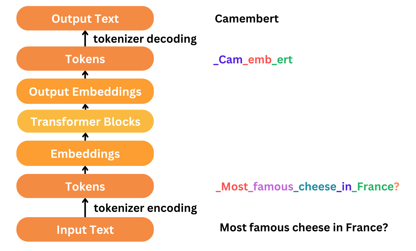
So in this article, we will try to understand the transformer architecture as defined in the paper and finally address the “transformer block” for our language translation model that we have seen in the diagram below.

100-feet view of Transformers

Over the course of this series we’ve seen how researchers tackled language translation with RNNs, then came LSTMs followed by the seq2seq architecture and finally encoder-decoder RNNs with attention which proved to be actually good at translation.

The challenge how was that the RNNs are notoriously difficult to train. Also passing context still proved to be a challenge since the RNNs unfold as the words are passed. This means that model has to do it sequentially and doesn’t know what relates to what until it actually sees the word!

The paper addresses both these concerns in one shot with the transformer architecture which allows for words to be processed in parallel and at each step of the way incorporate the context from all the words in the sequence. This proved to be quite the game changer since the model was not able to perform almost an order of magnitude faster while producing even better results!

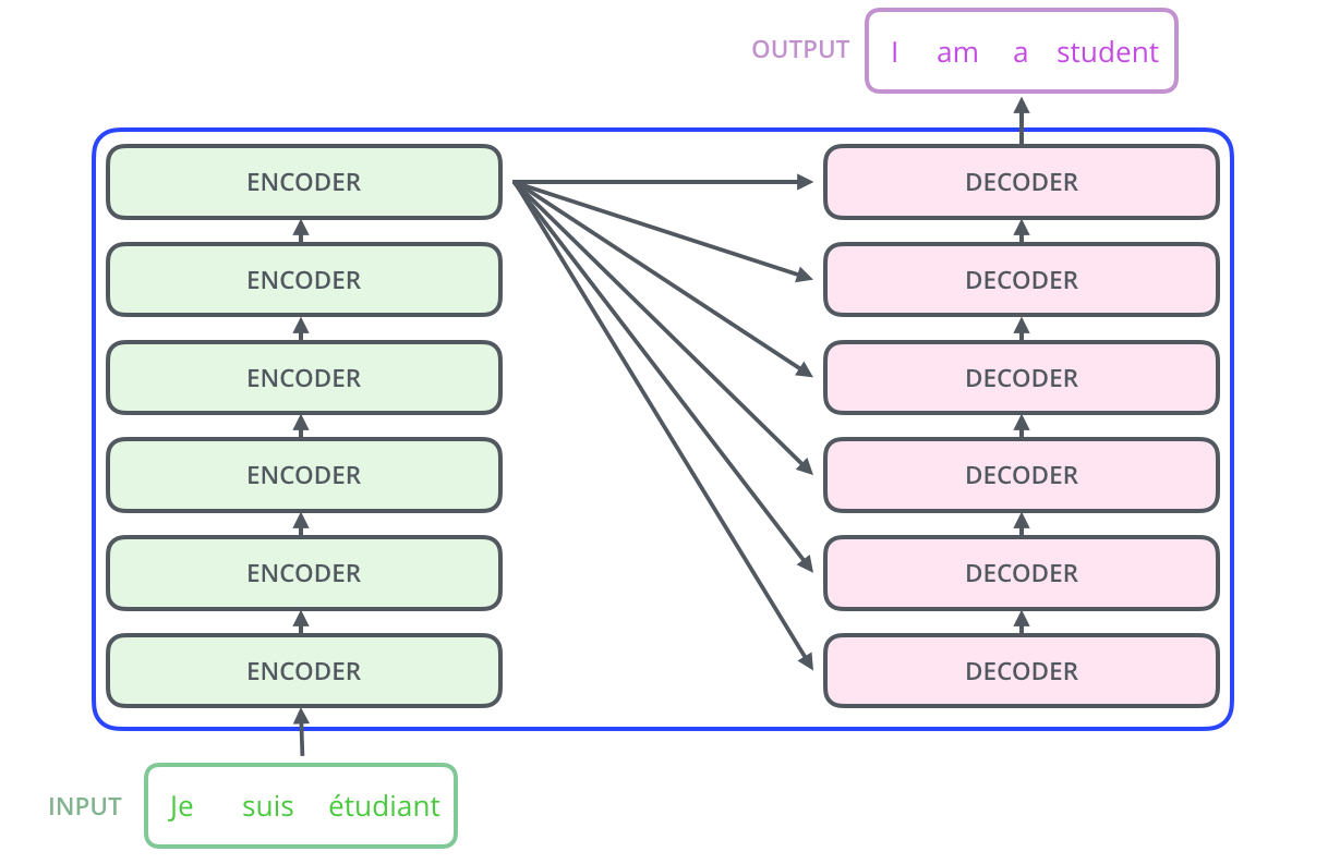
The transformer architecture looks pretty similar to the encoder-decoder where essentially there are two main blocks:

• Encoder
  • The encoder has lot of “transform blocks” stacked on top of each other
    • Similar to how we stacked LSTM units for the seq2seq
  • When we pass a sentence to a transformer block, the weights for block remain the same; just the word embeddings vary.
    • Again same as LSTMs
  • Each encoder layer passes it’s output to the next encoder layer above it
  • And you can stack multiple transformer blocks on each layer to model more complex relations
    • Again similar to LSTMs in seq2seq
• Decoder
  • The decoder again has a lot of “transform blocks” stacked on top of each other
  • The final output is a context vector to a fully connected MLP with a $softmax$
  • This returns the probability of each word in the vocab of the target language and we pick the one with the highest probability
  • The decoder keeps running until it outputs <EOS> or <SOS> (End-Of-Sentence or Start-Of-Sentence) based on how the transformer was trained.

Now it may seems like the encoder and decoder are similar which is true to an extent with a slight difference. The decoder has an additional step called encoder-decoder attention. Let’s looks at all these components:

• Self-Attention layer
  • It looks at all the input words and comes up with a context vector that contains information of each word and other words relevant to it.
  • Consider this sentence “The cat stopped, it looked angry”, the word it refers to the word cat which we know
  • The attention value of the word it will have context information of the word cat as well, that is what we mean by self-attention
  • To summarize, self-attention is when each word looks at every other word in the same sentence and compute a representation that accurately represents this
• Feed-Forward layer
  • It is a fully connected neural network that is added to handle large vocabulary and model complex relations.
  • That’s it!
• Encoder-Decoder attention
  • Here the decoder state of a word (which is the output from the decoder’s self-attention) looks at ALL the encoder states for any similarity or relation
  • This helps the decoder to translate the word with more context information

We have skipped a few components and steps but that’s fine since this captures the essence of transformers and what makes them so powerful. At every step of the way, the words have context information on the sentence itself and the source sentence which allows for very accurate translations.

The Transformer Model

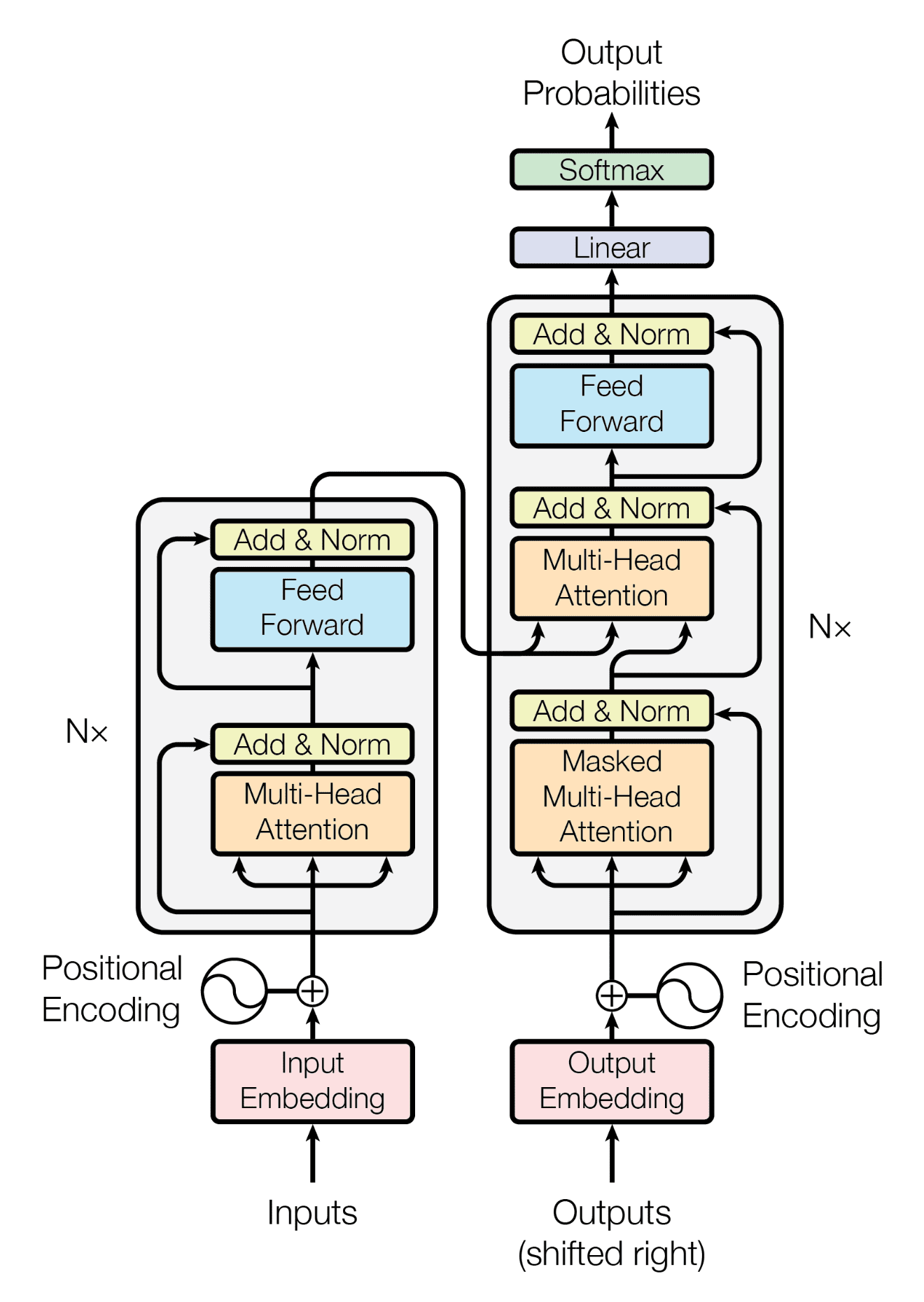
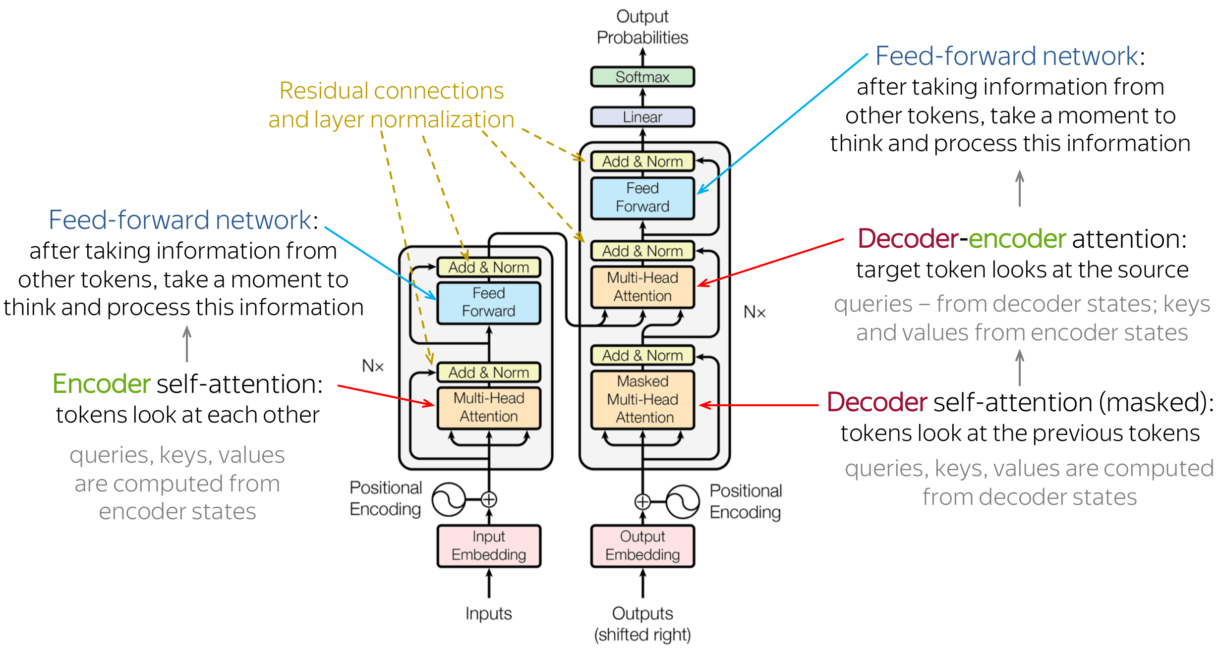
The paper defines the transformer block as shown below. We’ll look at each of the components in detail.

Input Embeddings

We have covered quite extensively in our previous posts how machines don’t understand words the way humans do. So we need a way to represent them in such a way where they can learn the grammar and semantics of the language. We do that via a combination of tokenization (break down sentences into tokens) and word embeddings (represents words to a lower dimensional space with semantic significance).

This is exactly what happens in the input and output embeddings where pass the sentence in source language to Input Embeddings and sentence in target language to Output Embeddings to get the respective word embeddings for training.

So now you’ve trained the model and you want to translate “Let’s go” to Spanish. We compute the word embeddings for ["let's", "go"] as part of Input Embedding but we don’t know the output sentence. So we start with <EOS> and pass its Output Embeddings to the decoder. The decoder outputs ["Vamos"] which we take, generate the embedding and pass back to the decoder (kind of like how we unfold a RNN). The decoder now outputs <EOS> which we know is the end of the sentence so we can conclude our inference.

Positional Encoding

As the name suggests, positional encoding is way to embed the position of the word in the sequence into the word itself. For example, the sentence “Cat eats fish” where reversed “Fish eats cat” means very different. So when we generate the word embedding for “cat” it doesn’t contain information of where this word appears in the given sequence! This is important information for the model to translate accurately.

Since Transformer does not contain recurrence (like in RNNs), it does not know the order of input tokens. Therefore, we have to let the model know the positions of the tokens explicitly.

The positional embeddings can be learned, but the authors found that having fixed ones does not hurt the quality. The fixed positional encodings used in the Transformer are: \(PE_{pos, 2i} = sine(pos/10000^{2i/d_{model}})\) \(PE_{pos, 2i+1} = cosine(pos/10000^{2i/d_{model}})\)

Where:

• $pos$ is the position of the word in the sequence (starting from 0)
• $i$ is the vector dimension (starting from 0)
• $d_{model}$ is the total number of dimensions in the model

These functions use sine for even dimensions and cosine for odd dimensions. Each dimension of the positional encoding corresponds to a $sinusoid$, and the wavelengths form a geometric progression from $2\pi$ to $10000\cdot2\pi$

The sinusoid works for transformer due to the following reasons:

1. Periodicity and Smoothness:
   • Sinusoidal functions are periodic and continuous, providing a smooth representation of positions. This periodicity helps the model generalize to longer sequences and ensures that the positional encoding can represent positions across a wide range of values.
2. Unique Representation:
   • Each position has a unique encoding, and similar positions have similar encodings, ensuring that the positional information is easily distinguishable. This unique mapping helps the model to learn positional relationships effectively.
3. Scale Invariance:
   • The use of different frequencies in the sine and cosine functions allows the model to capture information at different scales. Low-frequency components can capture long-range dependencies, while high-frequency components can capture short-range dependencies.
4. Compatibility with Addition:
   • By using trigonometric functions, the positional encodings can be easily added to the input embeddings without needing a separate mechanism for combining positional and content information. This addition maintains the input dimensionality and ensures seamless integration with the embeddings.

The final output to the encoder is a sum of the word embeddings and the positional embeddings for each token in the input sentence.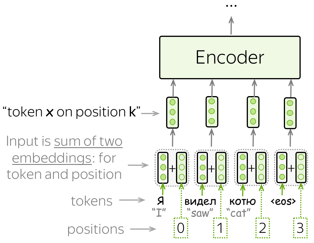

Encoder

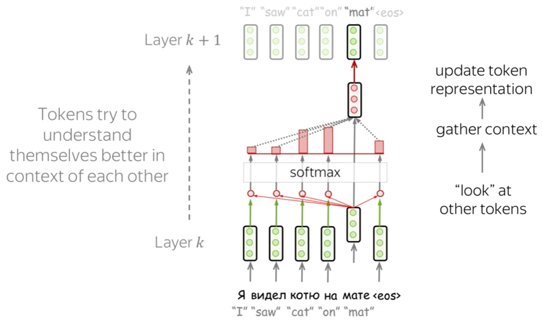
Intuitively, Transformer’s encoder can be thought of as a sequence of reasoning steps (layers). At each step, tokens look at each other (this is where we need attention - self-attention), exchange information and try to understand each other better in the context of the whole sentence. This happens in several layers (e.g., 6 as per the paper).

Self-Attention

Self-attention is one of the key components of the model. The difference between attention and self-attention is that self-attention operates between representations of the same nature: e.g., all encoder states in some layer.

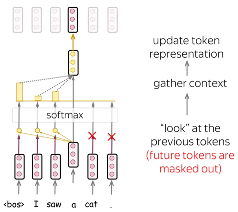
Self-attention is the part of the model where tokens interact with each other. Each token “looks” at other tokens in the sentence with an attention mechanism, gathers context, and updates the previous representation of “self” as shown in the diagram below.

Note that in practice, this happens in parallel.

Query, Key, and Value in Attention

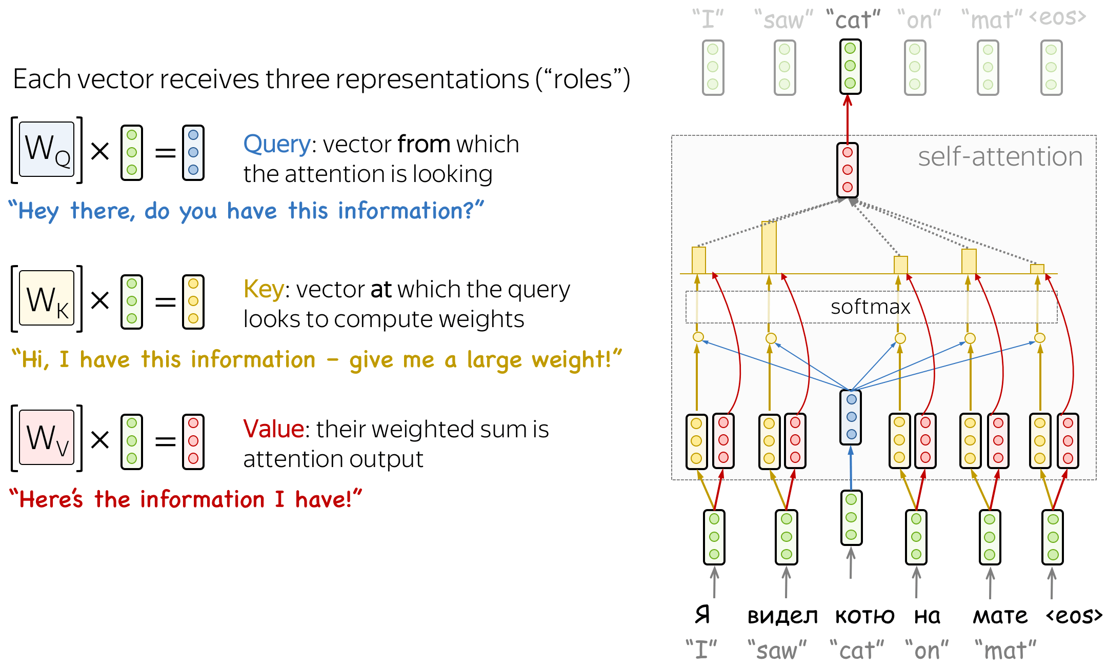
Formally, this intuition is implemented with a query-key-value attention. Each input token in self-attention receives three representations corresponding to the roles it can play:

• query - asking for information;
  • The query is used when a token looks at others
  • It’s seeking the information to understand itself better.
• key - saying that it has some information;
  • The key is responding to a query’s request
  • It is used to compute attention weights.
• value - giving the information.
  • The value is used to compute attention output
  • It gives information to the tokens which “say” they need it (i.e. assigned large weights to this token).

Given an input embedding for a word, these 3 vectors are computed using a fixed set of weights for the transformer block.

• Query vector $q$ will be used when we want to compare the word against the other words in the sentence.
• Key vector $k$ sole purpose is to respond to the query vector $q$
• $q$ and $k$ are used to compute the attention weights, which tell the important of each word in the sentence to the source word.
  • Normally, we expect a high weight for itself and other words based on grammar
  • For example, the attention weights for it in the sentence “The cat stopped and it looked angry” will have high weights for words it and cat
• The attention weights are combined with the value vector $v$ which contains the actual word information.

As per the paper, the formula for computing attention output is as follows:

Coming back to the example “The cat stopped and it looked angry” and if I want to compute the attention value of the word it:

• I have to compute $q_{it}$, $k_{it}$ and $v_{it}$ by multiplying the respective weights and the input embedding for it.
• Then I take the dot product of the query vector $q_{it}$ with the key vectors of all the other words $k_{the}, k_{cat}, k_{stopped}, k_{and} …$
• I take all these values and put it through a $softmax$ function which returns a value in the range of $[0,1]$ for each token (attention weights)
• We multiply these weights with the value vector of each of the words $v$ and add it all up to get the attention value for it $Attention(q_{it}, k_{it}, v_{it})$

Multi-Head Attention

Similar to how we can stack multiple LSTM units in a seq2seq, we can do the same with transformer blocks in the encoder as well. This allows the model to capture more complex relations and semantics which may not be sufficient with just 1 transformer block.

Usually, understanding the role of a word in a sentence requires understanding how it is related to different parts of the sentence. This is important not only in processing source sentence but also in generating target. For example, in some languages, subjects define verb inflection (e.g., gender agreement), verbs define the case of their objects, and many more. What I’m trying to say is: each word is part of many relations.

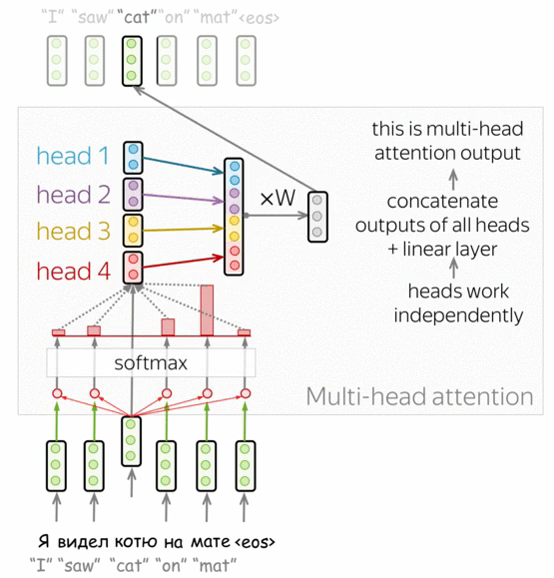
Therefore, we have to let the model focus on different things: this is the motivation behind Multi-Head Attention. Instead of having one attention mechanism, multi-head attention has several “heads” which work independently.

Mathematically, you can think of multi-head attention as attention values computed with different set of weights for query, key and value vectors to generate different attention scores for the same token. But finally we concatenate them and reduce it to a lower dimensional representation such that models with one attention head or several of them have the same size - multi-head attention does not increase model size.

Layer Normalization

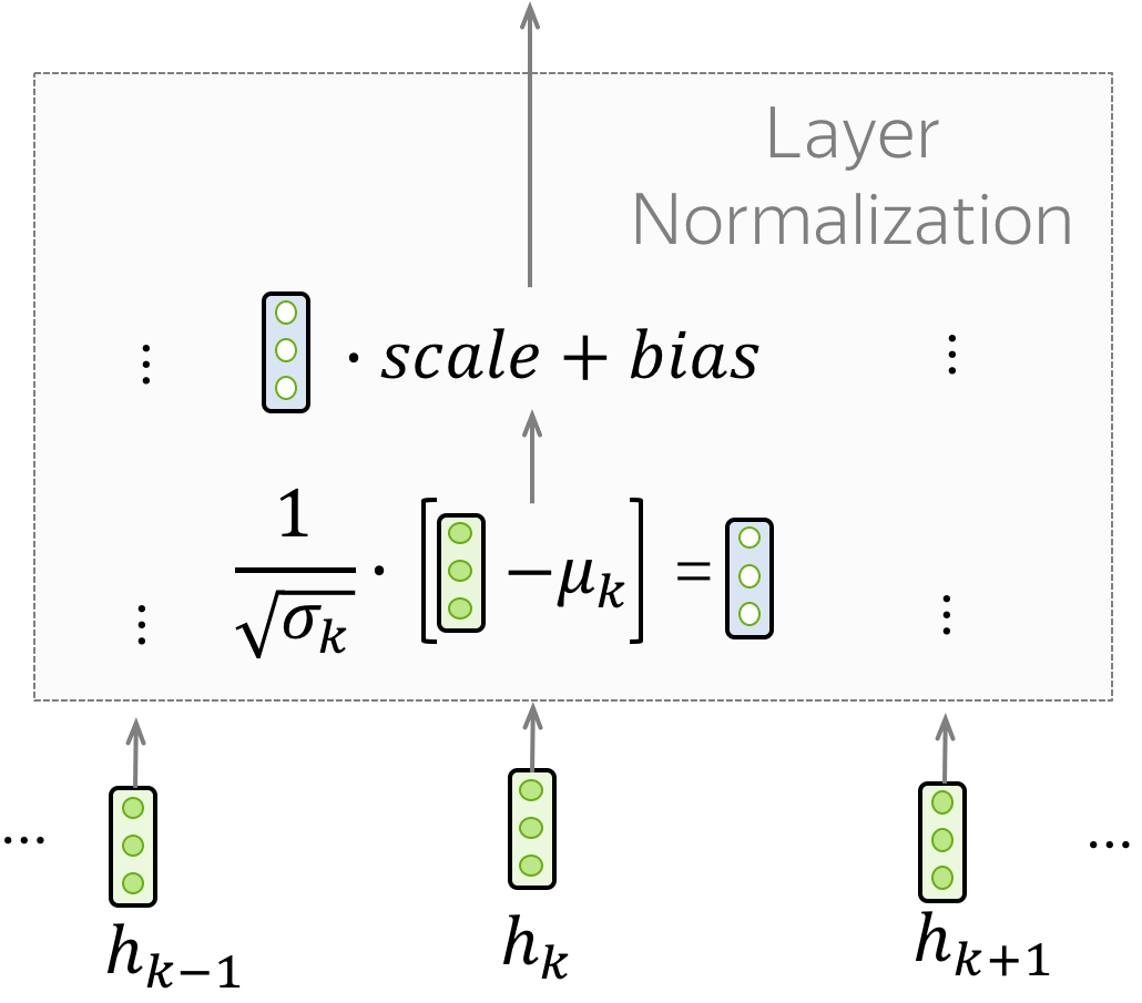
The ”Norm” part in the ”Add & Norm” layer denotes Layer Normalization. It independently normalizes vector representation of each example in batch - this is done to control “flow” to the next layer. Layer normalization improves convergence stability and sometimes even quality.

In the Transformer, you have to normalize vector representation of each token. Additionally, here LayerNorm has trainable parameters, $scale$ and $bias$, which are used after normalization to rescale layer’s outputs (or the next layer’s inputs).

Residual connections

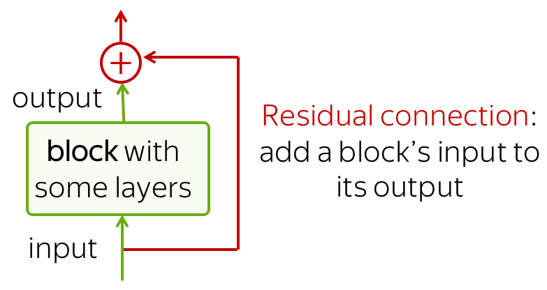
Residual connections are very simple (add a block’s input to its output), but at the same time are very useful: they ease the gradient flow through a network and allow stacking a lot of layers.

In the Transformer, residual connections are used after each attention and FFN block. On the earlier transformer illustration, residuals are shown as arrows coming around a block to the yellow ”Add & Norm” layer. In the ”Add & Norm” part, the ”Add” part stands for the residual connection.

Feed-Forward Neural Network (FFN)

After the attention values are computed for each word, we add the input embedding of the word itself back to the word’s attention value via a residual connection & normalize the final vector.

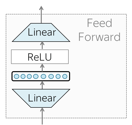
This vector is then passed as an input to the feed-forward neural network. Each transformer layer has a feed-forward network block: two linear layers with ReLU non-linearity between them: \(FFN(x) = max(0, xW_1 + b_1)W_2 + b_2\)

After looking at other tokens via an attention mechanism, a model uses an FFN block to process this new information (attention - ”look at other tokens and gather information”, FFN - ”take a moment to think and process this information”).

In other words, the FFN allows to model complex relationships based on the identified attention values. If attention values are the information, the FFN allows the model to learn how to use it efficiently.

Imagine you’re baking a cake. The self-attention mechanism is like gathering all the ingredients and understanding how they should interact based on the recipe (flour, sugar, eggs, etc.). But to actually make the cake, you need to process these ingredients—mixing, baking, and decorating them. This processing step is analogous to the feed-forward blocks in the Transformer.

To broadly list, FFN is important to the transformer for the following reasons:

• While self-attention layers help with capturing relationships and dependencies between different words in a sequence, they are inherently linear operations.
• They help in refining and re-representing the information captured by the self-attention mechanism
• The feed-forward network typically consists of two linear layers with a ReLU activation in between.
  • The first linear layer expands the dimensionality of the input, and the second linear layer reduces it back to the original size.
  • This expansion allows the model to operate in a higher-dimensional space temporarily, enabling it to capture more nuanced patterns before reducing back to the original size.
• By stacking multiple layers of self-attention and feed-forward networks, the Transformer gains depth, allowing it to learn hierarchical representations.
  • Deeper networks are generally more capable of capturing complex patterns and abstractions in the data.

Decoder

In each decoder layer, tokens of the prefix also interact with each other via a self-attention mechanism, but additionally, they look at the encoder states (without this, no translation can happen, right?).

Masked Multi-Head Attention

In the decoder, there’s also a self-attention mechanism: it is the one performing the “look at the previous tokens” function.

In the decoder, self-attention is a bit different from the one in the encoder. While the encoder receives all tokens at once and the tokens can look at all tokens in the input sentence, in the decoder, we generate one token at a time: during generation, we don’t know which tokens we’ll generate in future.

To forbid the decoder to look ahead, the model uses masked self-attention: future tokens are masked out. Look at the illustration.

During generation, it can’t - we don’t know what comes next. But in training, we use reference translations (which we know). Therefore, in training, we feed the whole target sentence to the decoder but without masks, the tokens would “see future”, and this is not what we want.

The Transformer does not have a recurrence, so all tokens can be processed at once. This is one of the reasons it has become so popular for machine translation - it’s much faster to train than the once dominant recurrent models. For recurrent models, one training step requires O(len(source) + len(target)) steps, but for Transformer, it’s O(1), i.e. constant !!

Cross Attention

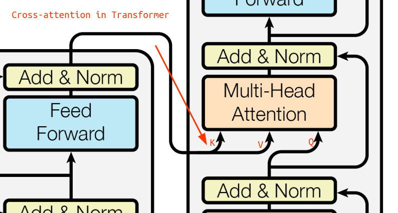
Cross attention, also known as encoder-decoder attention, is very similar to the self-attention in the encoder with a very small twist. The decoder needs to learn how to convert the encoder output to the target language so it makes sense that it needs to pay attention to the encoder’s representation of the source words while also paying attention to itself.

That’s exactly what happens in the decoder. First it pays attention to sequence in the translated language via a Masked Self-Attention layer and then taken this information to compute an attention score comparing against the encoder’s key and value vectors.

Let’s try to understand cross attention from the diagram above:

• Intuitively, we know we are trying to understand if a word embedding in the decoder needs to pay attention to any of the words in the encoder sequence
• In attention, to query we use the q vector and since we want to query for the decoder’s word we use the q from the decoder
  • We compute a new $q$ vector based on the next context vector (output from self-attention, add & norm) & the query vector weights $W_q$
• To query against, we need to compute the similarity score against the key vectors k of the encoder words which results in a bunch of cross-attention weights ($q$ from decoder $\odot$ $k$ from encoder)
  • Again we have different context vectors as an output from multiple layers of transformers, feed forward neural nets, add and normalization
  • We just multiple each of these context vectors with the top layer’s key and value weights ($W_k$ and $W_v$)
  • We use these newly computed key and value vectors for attention computation
• Finally, we multiple the weights with the value vectors for all the words in the encoder & sum it up to get the cross attention value for the decoder word!

Summary

The transformer architecture is very powerful and has inspired many more popular models like BERT, GPT2, GPT3, LLaMa etc. The below diagram summarizes our understanding of transformers.

Further Readings

• https://www.youtube.com/watch?v=PSs6nxngL6k&list=PLblh5JKOoLUIxGDQs4LFFD–41Vzf-ME1&index=19&ab_channel=StatQuestwithJoshStarmer
• https://lena-voita.github.io/nlp_course/seq2seq_and_attention.html#attention_intro
• https://jalammar.github.io/visualizing-neural-machine-translation-mechanics-of-seq2seq-models-with-attention/
• https://research.google/blog/transformer-a-novel-neural-network-architecture-for-language-understanding/
• https://web.stanford.edu/~jurafsky/slp3/10.pdf
• https://www.youtube.com/watch?v=iDulhoQ2pro
• https://www.kaggle.com/code/soupmonster/attention-is-all-you-need-pytorch
• https://nlp.seas.harvard.edu/annotated-transformer/
• https://d2l.ai/chapter_attention-mechanisms-and-transformers/index.html
• Paper - Attention is all you need
• https://www.youtube.com/watch?v=eMlx5fFNoYc&ab_channel=3Blue1Brown
• ChatGPT