LLMs Series - Part 5 - Attention!

Issue with LSTM encoder-decoder

LSTMs were a good step forward towards machine translation but it had its short comings. If you want to just translate a sentence or two, it performs well but say you want to translate a paragraph or a book, the LSTM encoder-decoder falters!

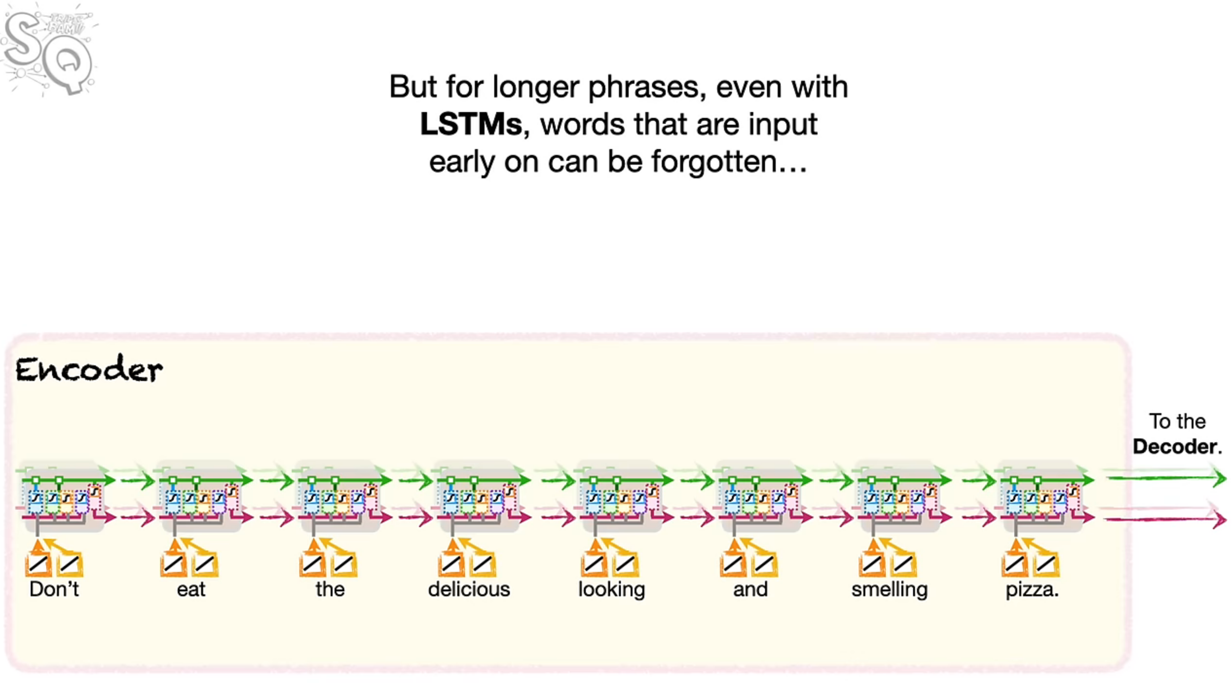
Even for long phrases, the words that are passed early on are forgotten by the time it’s passed to the decoder. And if the first word is forgotten in the example above, the translated sentence might mean entirely different!

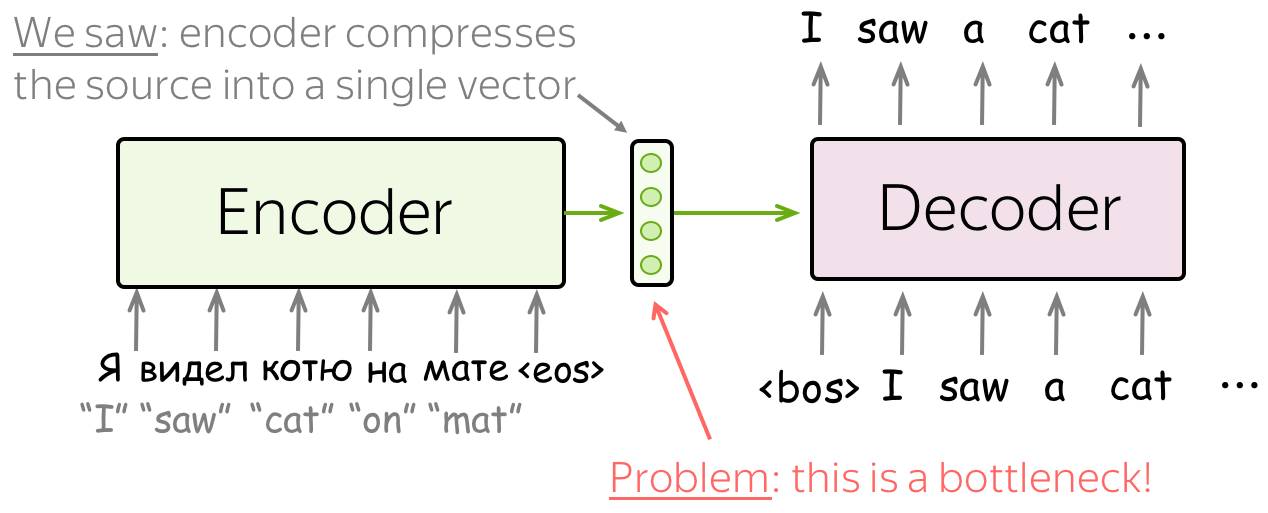
So why is the encoder-decoder LSTM unable to remember the words passed early on? The issues seems to be the context vector. We compress all the information in the input sequence into a single vector which may not be capable of capturing all the information.

Not only it is hard for the encoder to put all information into a single vector - this is also hard for the decoder. The decoder sees only one representation of source. However, at each generation step, different parts of source can be more useful than others. But in the current setting, the decoder has to extract relevant information from the same fixed representation - hardly an easy thing to do.

Attention Mechanism

Attention was introduced in the paper Neural Machine Translation by Jointly Learning to Align and Translate to address the fixed representation problem.

Let’s try to intuitively understand attention. The decoder is try to decode from the context vector the translation for “I saw a cat on the mat”. Now image if the decoder can some how look back at the parts which are necessary for translation. For generating the first output, the decoder can look at “I”, “saw” and the context vector to generate “j’ai”, for the next word it looks at the updated context vector and “saw” to generate “vu” and so on. This overcomes the limitation of the context vector by allowing the decoder to look back at selective parts of the encoder.

An attention mechanism is a part of a neural network. At each decoder step, it decides which source parts are more important. In this setting, the encoder does not have to compress the whole source into a single vector - it gives representations for all source tokens (for example, all RNN states instead of the last one).

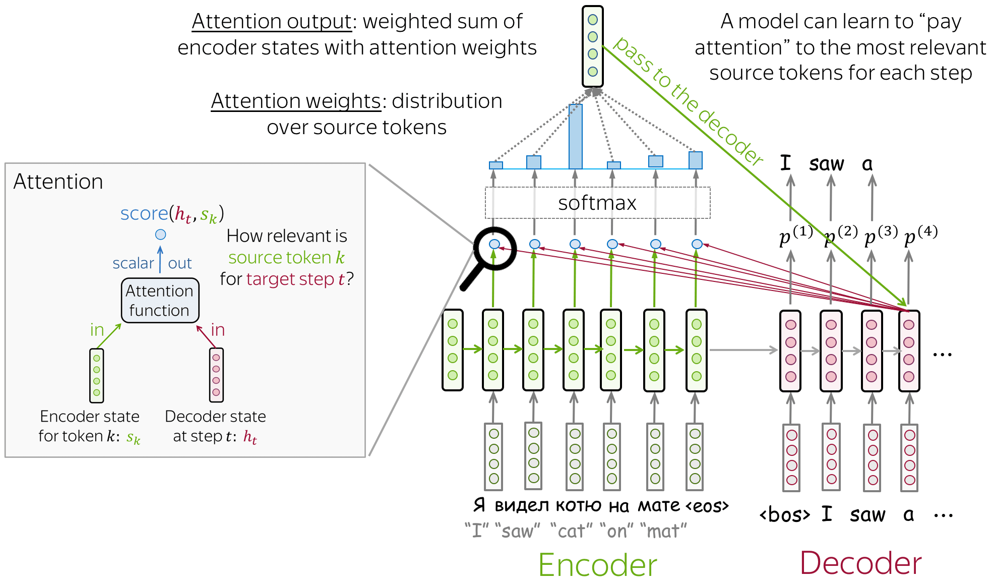
At each decoder step, attention

• receives attention input: a decoder state $h_t$ and all encoder states $s_1, s_2, .. s_m$
• computes attention scores
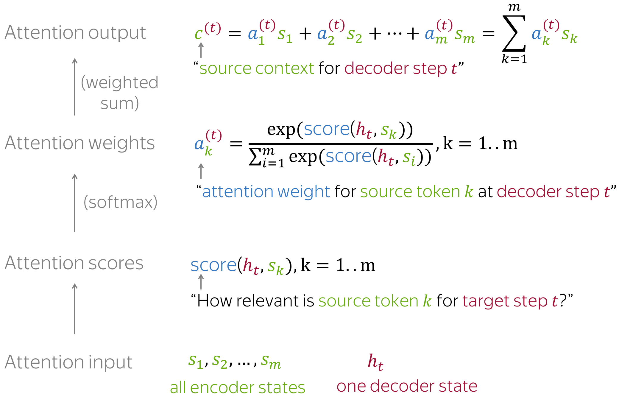
  For each encoder state $s_k$, attention computes its “relevance” for this decoder state $h_t$. Formally, it applies an attention function which receives one decoder state and one encoder state and returns a scalar value $score(h_t, s_k)$;
• computes attention weights: a probability distribution - $softmax$ applied to attention scores;
• computes attention output: the weighted sum of encoder states with attention weights.

The general computation is as follows:

The attention output contains relevant context information for $h_t$ which is the decoder LSTM unit’s output. This attention output is passed along with the decoder output $h_t$ to a fully connected layer with a $softmax$ to generate a word embedding in the translated language.

Since everything here is differentiable (attention function, softmax, and all the rest), a model with attention can be trained end-to-end. You don’t need to specifically teach the model to pick the words you want - the model itself will learn to pick important information.

Attention Model Variants

As specified earlier, the attention score is a measure of how relevant the source token $s_k$ is to the the target step $t$ with decoder output as $h_t$. There are a number of ways to compute this score function. One of the simplest ways is to define $score(h_t, s_k)$ as a similarity function between the two vectors, for example, cosine similarity which can often be approximated to a dot product.

Geometrically, cosine similarity only cares about angle difference, while dot product cares about angle and magnitude. If you normalize your data to have the same magnitude, the two are indistinguishable.

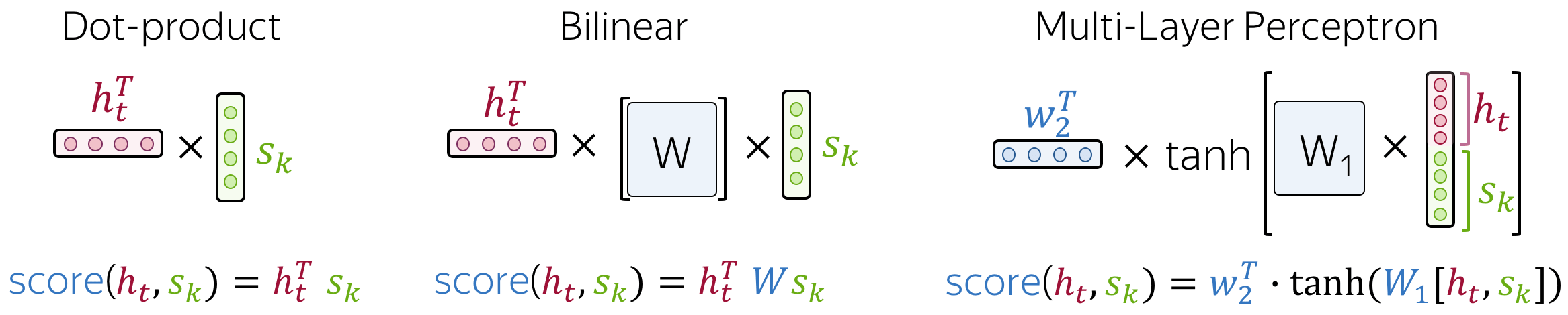
The most popular ways to compute attention scores are:

• dot-product - the simplest method;
• bilinear function (aka “Luong attention”) - used in the paper Effective Approaches to Attention-based Neural Machine Translation;
• multi-layer perceptron (aka “Bahdanau attention”) - the method proposed in the original paper.

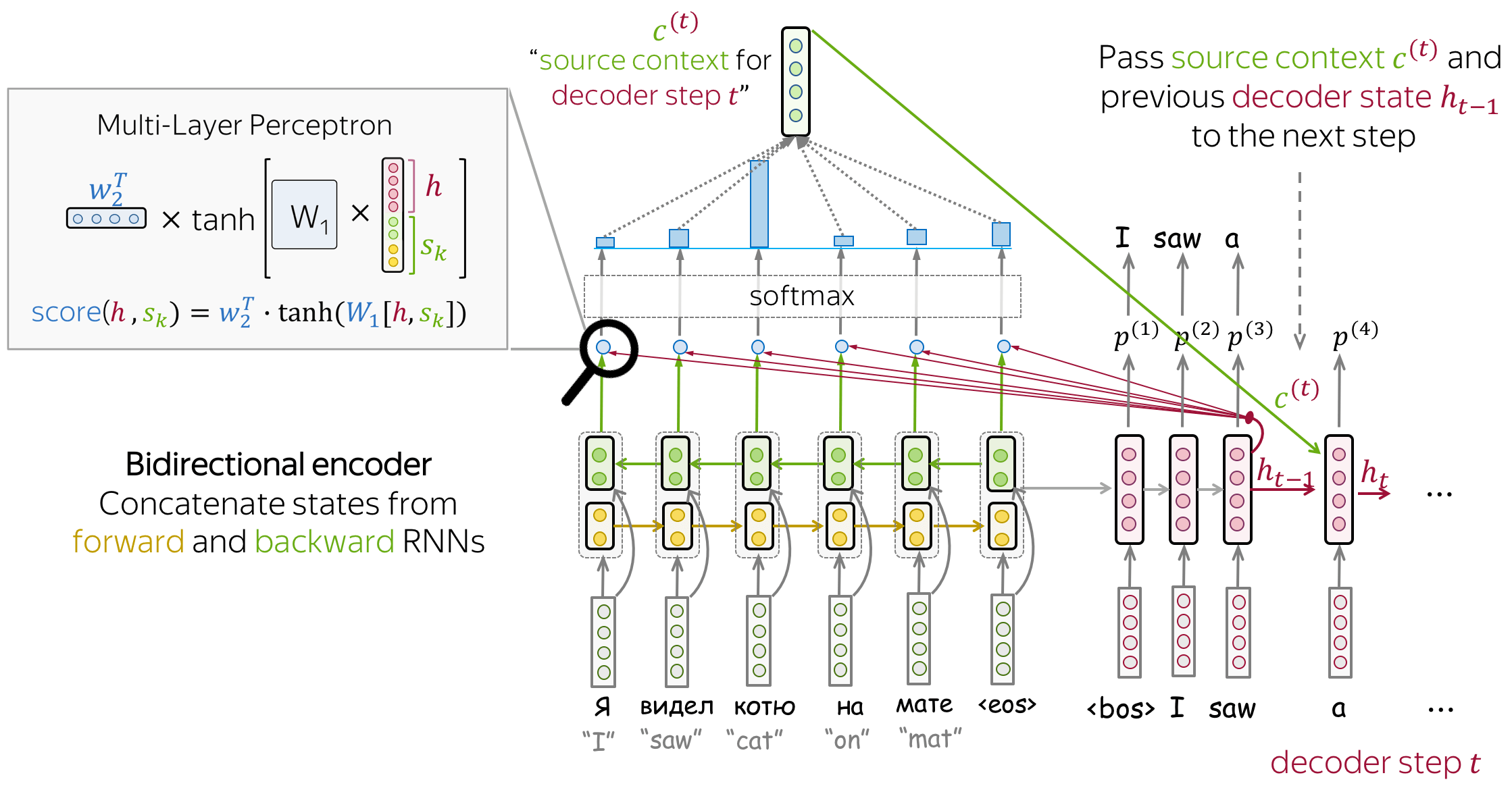
Bahdanau Model

• encoder: bidirectional
  To better encode each source word, the encoder has two RNNs, forward and backward, which read input in the opposite directions. For each token, states of the two RNNs are concatenated.
• attention score: multi-layer perceptron
  To get an attention score, apply a multi-layer perceptron (MLP) to an encoder state and a decoder state.
• attention applied: between decoder steps
  Attention is used between decoder steps: state $ℎ_{𝑡−1}$ is used to compute attention and its output $c^{(t)}$, and both $h_{t-1}$ and $c^{(t)}$ are passed to the decoder at step $t$.

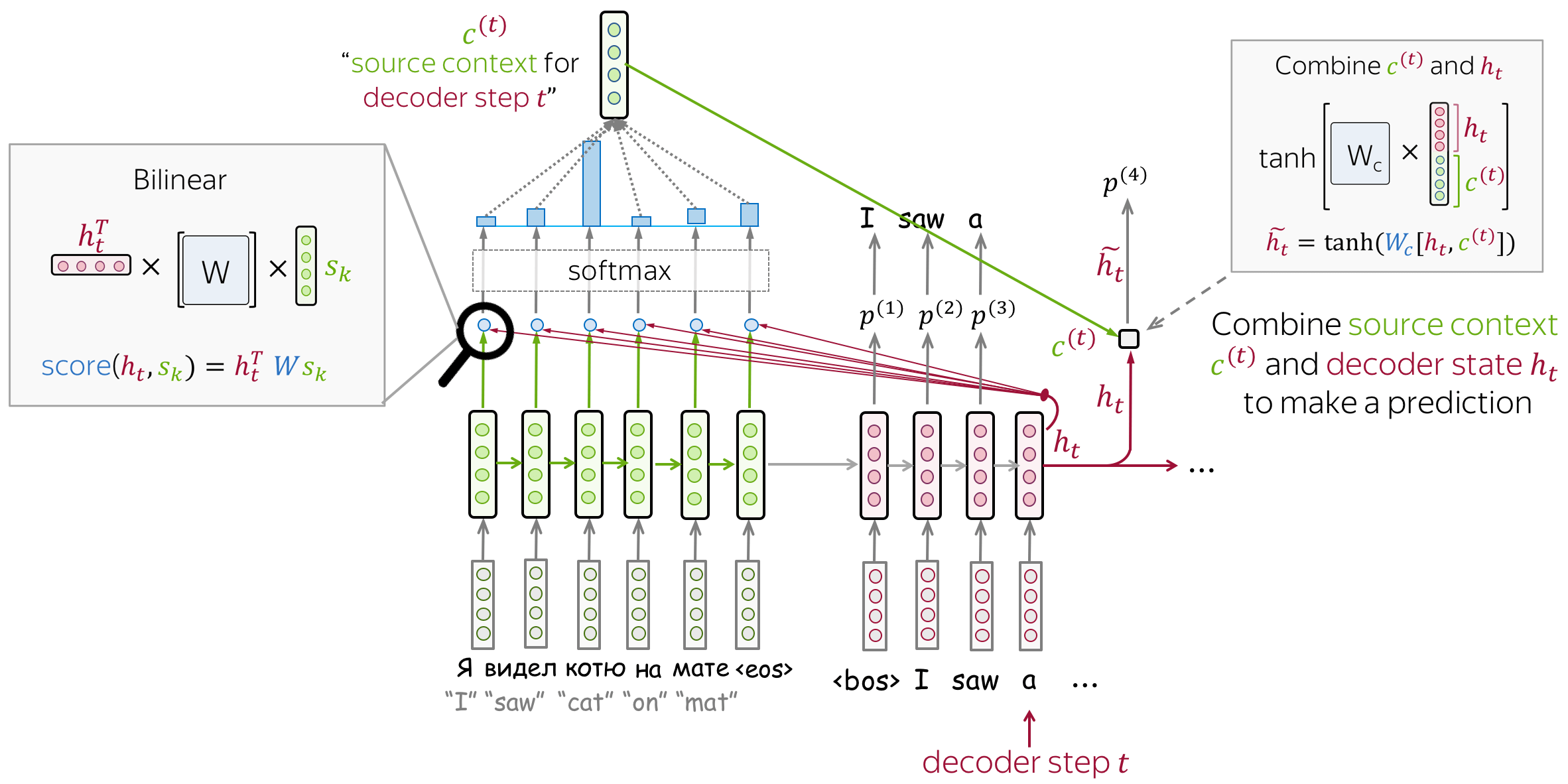
Luong Model

• encoder: unidirectional (simple)
• attention score: bilinear function
• attention applied: between decoder RNN state 𝑡 and prediction for this step
  Attention is used after RNN decoder step 𝑡 before making a prediction. State $h_t$ used to compute attention and its output $c^{(t)}$. Then $h_t$ is combined with $c^{(t)}$ to get an updated representation $\tilde{h_t}$, which is used to get a prediction.

Further Readings

• https://www.youtube.com/watch?v=PSs6nxngL6k&list=PLblh5JKOoLUIxGDQs4LFFD–41Vzf-ME1&index=19&ab_channel=StatQuestwithJoshStarmer
• https://lena-voita.github.io/nlp_course/seq2seq_and_attention.html#attention_intro
• https://jalammar.github.io/visualizing-neural-machine-translation-mechanics-of-seq2seq-models-with-attention/
• ChatGPT