LLMs Series - Part 3 - RNNs

Posted Jun 1, 2024

By Allen Philip J 16 min read

Overview

In the previous parts, we covered how to tokenize the data & create word embeddings for training a large language model (LLM). Now let’s look into the model architecture itself.

In this article, we’ll look in detail at RNNs which are a powerful variant of neural networks that aim the preserve context. This set the context to answer how early NLMs were designed via the seq2seq model architecture which we will look at in the next post.

To start with, let’s look at one of the most popular use cases of LLMs in the space of NLP, translation! Many of us may have used Google Translate at some point. It has become such an essential feature that is used almost without a second thought. In this article, we will attempt to see how this problem statement was tackled over the course of time.

Rule-Based Machine Translation (RBMT)

Era: 1950s-1980s

Approach:

Rule-Based Systems: These systems relied on manually crafted linguistic rules and dictionaries to translate text from one language to another.
Syntax and Semantics: They focused on parsing sentences based on grammatical structures and applying transformation rules to generate translations.

Strengths:

Human Expertise: Leveraged deep linguistic knowledge and human expertise.
Consistency: Produced consistent translations for well-defined grammatical structures.

Weaknesses:

Scalability: Difficult to scale due to the need for extensive rule creation for each language pair.
Complexity: Struggled with the nuances of natural language and idiomatic expressions.

Statistical Machine Translation (SMT)

Era: 1990s-2010s

Approach:

Data-Driven: SMT models used large parallel corpora (aligned bilingual texts) to learn translation probabilities.
Phrase-Based Models: Instead of word-for-word translation, SMT models translated phrases, capturing more context.
Alignment Models: Techniques like the IBM alignment models were developed to align words and phrases between source and target languages.

Key Algorithms:

Word Alignment: Giza++ and the IBM models.
Phrase-Based Translation: Moses, a widely used SMT toolkit.

Strengths:

Automation: Reduced the need for manual rule creation.
Adaptability: Could be adapted to new languages and domains by training on relevant corpora.

Weaknesses:

Data Dependency: Required large amounts of parallel data.
Quality Issues: Struggled with long-distance dependencies and nuanced language structures.

Neural Machine Translation (NMT)

Era: 2014-present

Neural networks were first introduced in 1950s but it remained largely theoretical and impractical at the time. The first breakthrough when the famous 1986 paper was published introducing the concept of “backpropogation” which allowed us to train neural networks. But still this space of research was largely dormant due to high computational requirements to train neural networks. All that changed in 2010s with the boom in GPUs which allowed for easily training their neural networks. With time came the deep neural networks in the form of AlexNet, ImageNet etc which revolutionized the field of computer vision and it has not lost steam since then.

Now let’s look at how neural networks help advance the field of NLP by tackling the machine translation problem.

Approach:

Deep Learning: NMT models use neural networks to learn the translation task end-to-end.
Encoder-Decoder Architecture: An encoder processes the source sentence into a fixed-size context vector, and a decoder generates the target sentence from this vector.
Sequence-to-Sequence Models: Introduced by Sutskever et al. in 2014, these models transformed how translation systems were designed.

Key Innovations:

Attention Mechanisms: Proposed by Bahdanau et al. in 2015, attention allows the model to focus on different parts of the source sentence during translation, improving handling of long sentences and complex structures.
Transformer Architecture: Introduced by Vaswani et al. in 2017, transformers use self-attention mechanisms to handle dependencies without recurrent networks, leading to significant performance improvements.

Before we jump into attention and transformer architectures, in this article we will focus on the different seq2seq models that has shaped the NLP domain.

Recurrent Neural Networks (RNNs)

Neural Networks are great but there posed a critical problem for machine translation which is remembering context which is an essential part of machine translation. To understand this let’s take an example where we are attempting to translate a sentence from English to French, “The chicken didn’t cross the road because it was scared”. When the model is translating, how does it know what “it” refers to? The need for context becomes more important when we are dealing with sentence completion, summarization, QA etc.

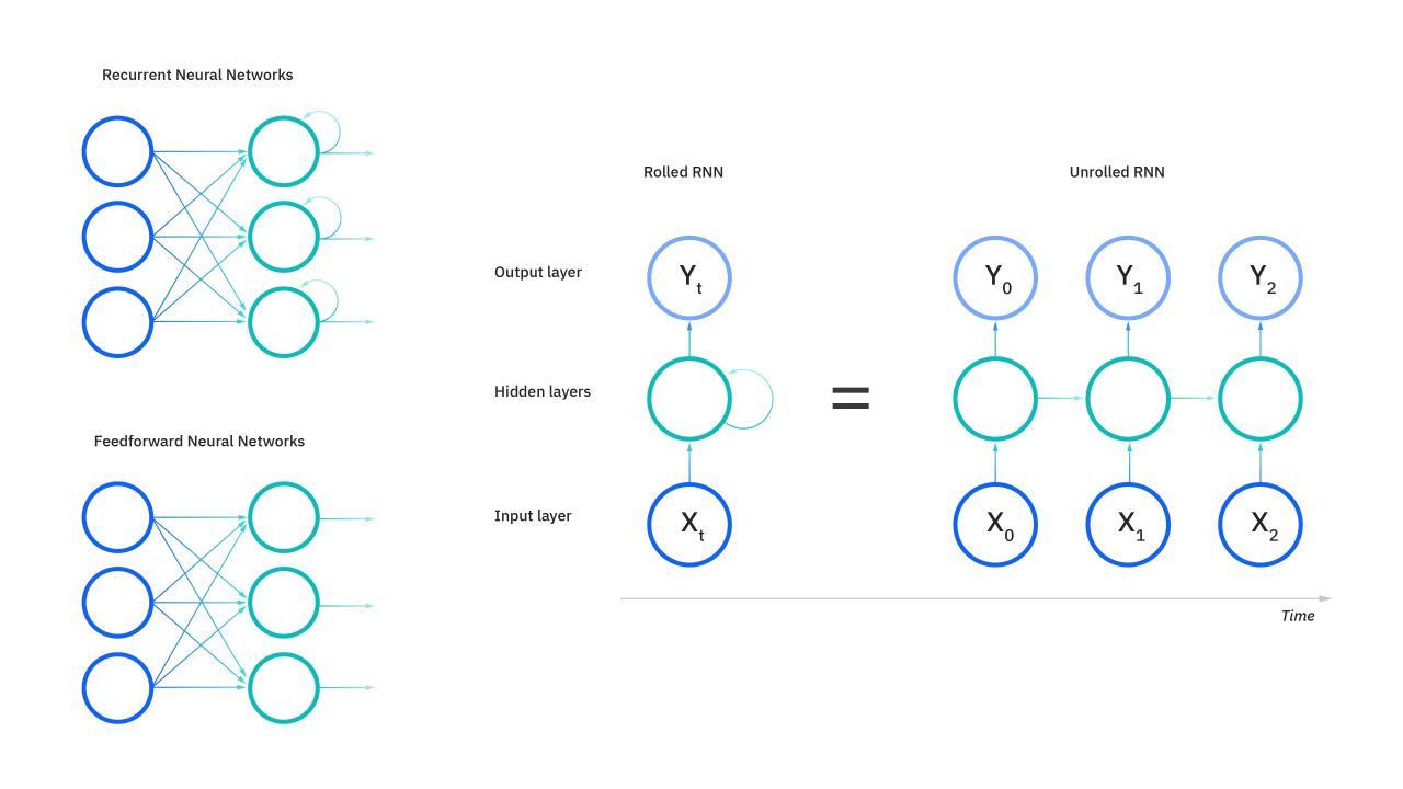
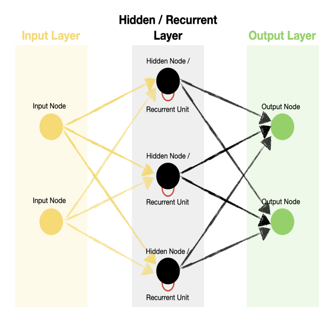
RNNs are designed to handle sequential data where the order of data points matters (e.g., time series, sentences). Unlike feed forward neural networks (ie, output from layer 1 is always fed forward to layer 2 and so on) which process inputs independently, RNNs maintain a hidden state that captures information from previous inputs in the sequence.

So what does this hidden state represent? Simply put it acts as a memory of the previous step. And this hidden state is updated based on the current input and the previous hidden state using a recurrent function.

Let’s understand this better with an example where we want to translate “The cat is on the mat”. We want to build a RNN which takes in 3 words and predicts the next word. For the example, we would break it down into words ["the", "cat", "is", "on", "the", "mat"] and generate labels like:

X = ["the", "cat", "is"], Y = "on"
X = ["cat", "is", "on"], Y = "the"
X = ["is", "on", "the"], Y = "mat"

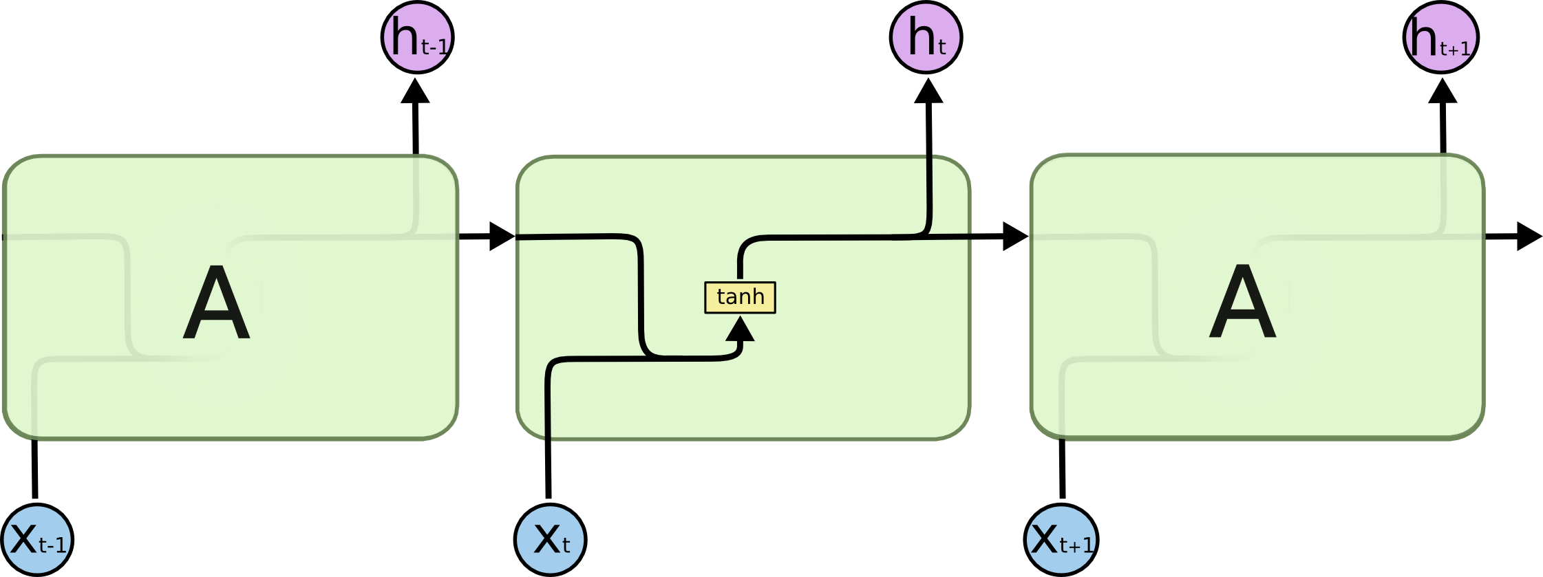
If you’re passing it to a RNN, we pass the sequence itself as input to the model in the order [x0, x1, x2] to allow the model to capture the context. As show in the diagram, first x0 is passed as input to RNN, the output of which is passed back as input back to the same layer . This is called as unrolling/unfolding of RNN as shown in the diagram above.

So x0 is passed to the first layer with hidden state h0 , the output is passed along with x1 to the next layer with hidden state h1 and so on. The output of first layer contains context information since it’s taking x0 as input.

Another distinguishing characteristic of recurrent networks is that they share parameters across each layer of the network. While feedforward networks have different weights across each node, recurrent neural networks share the same weight parameter within each layer of the network. This is because essentially we are just unrolling the same layer over and over again as shown below.

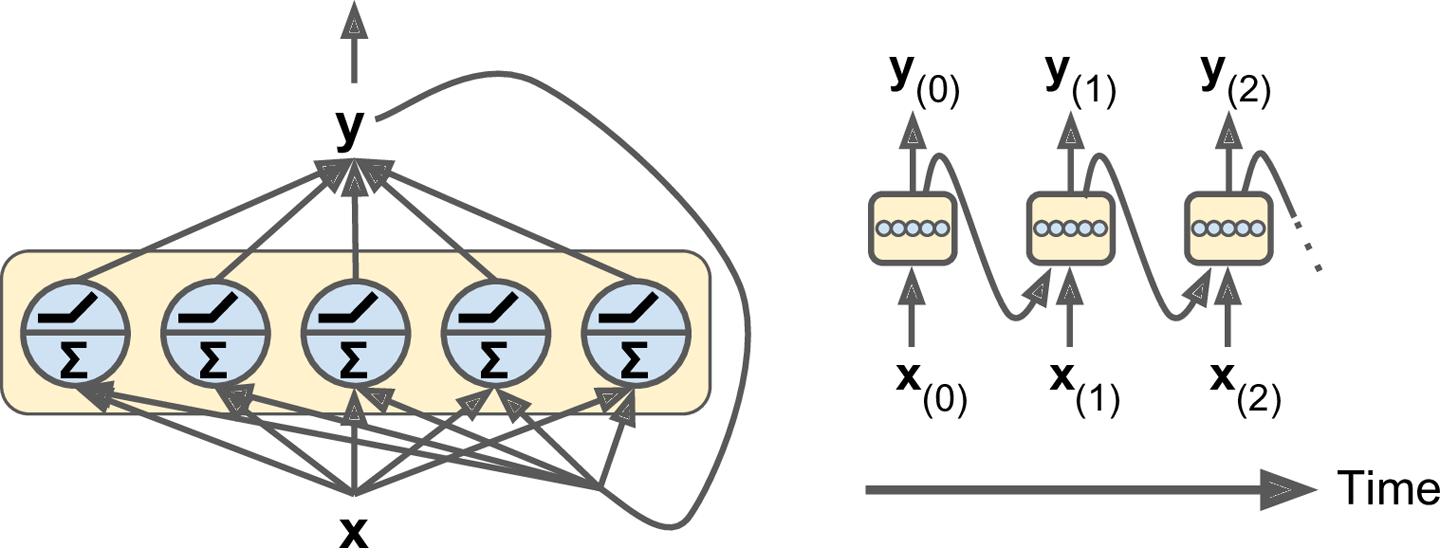
The above examples are an oversimplification of how a RNN might look since in practice it can have 100s of units which unfold into a softmax function to predict. As shown in the example below, we have multiple RNN units which unroll as many inputs being passed to them (in this case twice) and all the outputs are passed to an output node probably over a softmax.

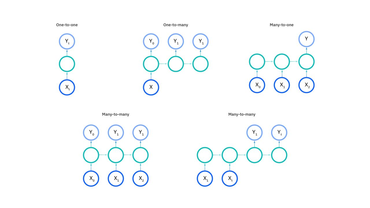
Feedforward networks map one input to one output, but RNNs do not actually have this constraint. Instead, their inputs and outputs can vary in length, and different types of RNNs are used for different use cases, such as music generation, sentiment classification, and machine translation.

The intuition behind RNNs lies in their ability to retain and propagate information through time steps, allowing them to learn dependencies and patterns in sequential data.

Capturing Dependencies:
- By maintaining a hidden state that gets updated at each time step, RNNs can capture dependencies between elements of a sequence, which is crucial for tasks like language modeling and time series prediction.
Memory Effect:
- The hidden state acts like a memory that retains information about previous inputs, enabling the network to use past context to inform future predictions.

RNNs proved to be better alternatives to feed forward neural networks for machine translation but not without it’s limitations:

Vanishing and Exploding Gradients:
- During backpropagation, gradients can either become very small (vanishing gradients) or very large (exploding gradients), making it difficult to train the network for long sequences.
- This limitation led to the development of more advanced architectures like LSTMs and GRUs.
Long-Term Dependencies:
- Standard RNNs struggle with capturing long-term dependencies due to the gradient issues mentioned above.

Long-Short Term Memory (LSTMs)

Long short-term memory (LSTM) is an RNN variant that enables the model to expand its memory capacity to accommodate a longer timeline. An RNN can only remember the immediate past input. It can’t use inputs from several previous sequences to improve its prediction.

Consider the following sentences: Tom is a cat__. Tom’s favorite food is fish. When you’re using an RNN, the model can’t remember that Tom is a cat. It might generate various foods when it predicts the last word. LSTMs are explicitly designed to avoid the long-term dependency problem. Remembering information for long periods of time is practically their default behavior, not something they struggle to learn!

All recurrent neural networks have the form of a chain of repeating modules of neural network. In standard RNNs, this repeating module will have a very simple structure, such as a single $tanh$ layer.

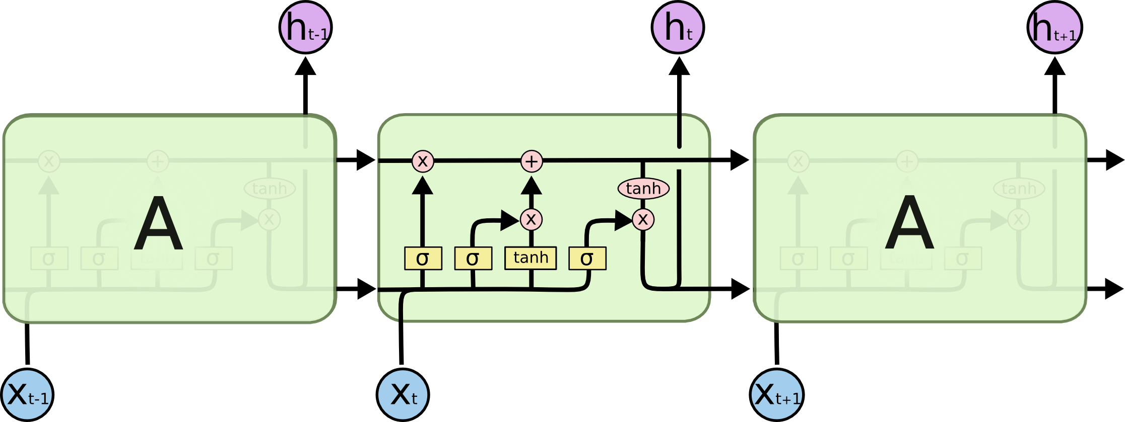
LSTMs also have this chain like structure, but the repeating module has a different structure. Instead of having a single neural network layer, there are four, interacting in a very special way.

Don’t worry about the details of what’s going on. We’ll walk through the LSTM diagram step by step later. For now, let’s just try to get comfortable with the notation we’ll be using.

The key to LSTMs is the cell state, the horizontal line running through the top of the diagram. It runs straight down the entire chain, with only some minor linear interactions. It’s very easy for information to just flow along it unchanged. This serves as a means to capture the long-term memory.

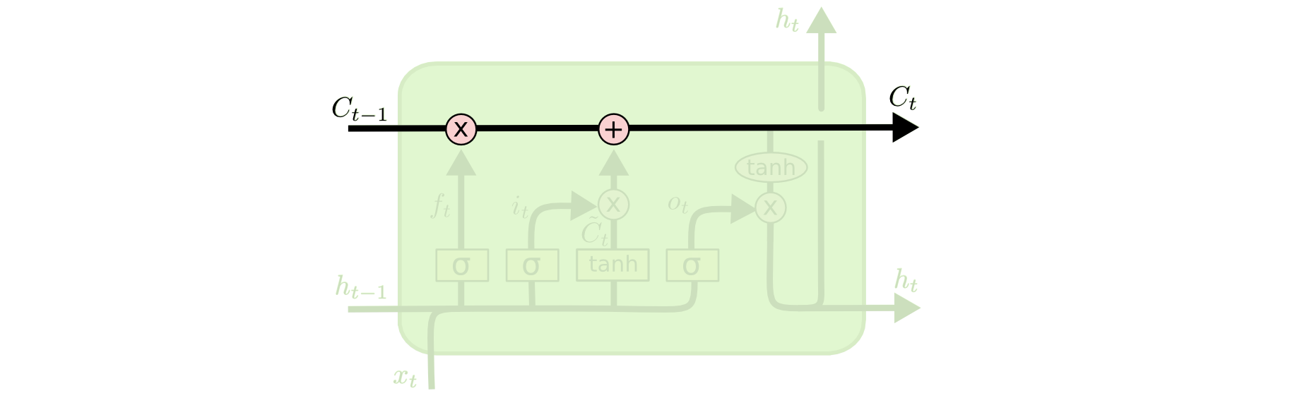
Now that we know the long-term memory can be propagated, the next question is how is it regulated or manipulated within a LSTM cell. This is done so by structures called as gates. Gates are a way to optionally let information through. They are composed out of a sigmoid neural net layer and a pointwise multiplication operation.

Step-by-Step LSTM Walkthrough

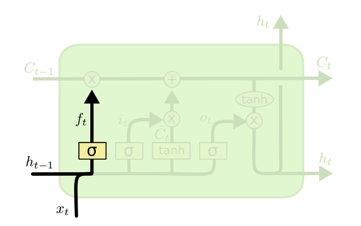
The first step in our LSTM is to decide what information we’re going to throw away from the cell’s long term state memory. This decision is made by a sigmoid layer called the “forget gate layer.”

A $sigmoid$ function, represented here as $\sigma$ block, is a mathematical function that always outputs a value in the range of $[0,1]$. Intuitively, this can be interpreted as function which defines how much percentage of the values to select, kind of like a logic gate, except it outputs a continuous value.

A $tanh$ function outputs a values in the range of $[-1,1]$. Intuitively in the context of LSTMs, we can interpret $tanh$ as a function that brings the values (whatever be the input ranges) to the target range of $[-1,1]$ and is typically used for the outputs of the LSTM (long-term $C_t$ and short-term $h_t$ memory states)

Let’s go back to our example of a language model trying to predict the next word based on all the previous ones. In such a problem, the cell state $C_{T-1}$ might include the gender of the present subject, so that the correct pronouns can be used. When we see a new subject, we want to forget the gender of the old subject. In the diagram below, $f_t$ represents how much of the previous cell state to remember (though it’s called the forget gate).

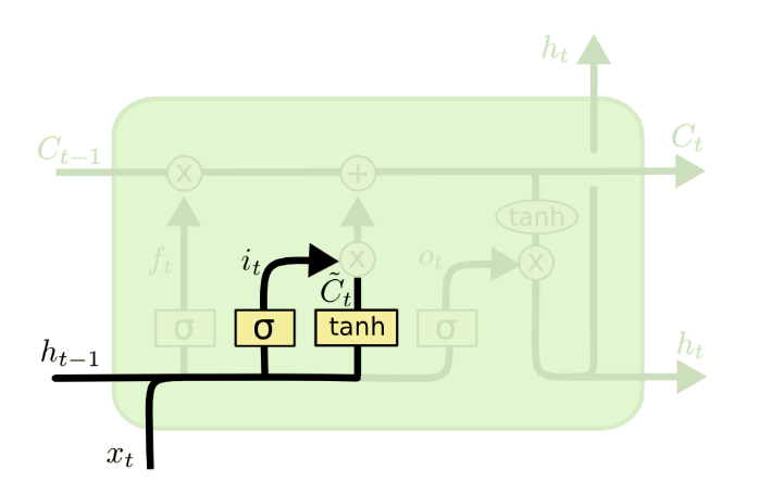
The next step is to decide what new information we’re going to store in the cell state. This has two parts. First, a sigmoid layer called the “input gate layer” decides which values we’ll update. Next, a $tanh$ layer creates a vector of new candidate values, $\tilde{C_t}$ that could be added to the state. In the next step, we’ll combine these two to create an update to the state. The purpose of this step is to prepare the variables that’ll be used to update the cell state $C_t$

In the example of our language model, we’d want to add the gender of the new subject to the cell state, to replace the old one we’re forgetting.

It’s now time to update the old cell state, $C_{t-1}$ into the new cell state $C_t$. The previous steps already decided what to do, we just need to actually do it.

We multiply the old state by $f_t$ forgetting the things we decided to forget earlier. To this value, we add $i_t * \tilde{C_t}$ which is the new candidate values scaled by how much we decided to update each state value.

In the case of the language model, this is where we’d actually drop the information about the old subject’s gender and add the new information, as we decided in the previous steps.

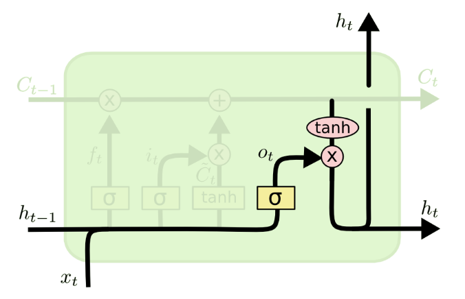
So far we have updated the cell state, now we need to generate the actual output (short-term memory state) of the LSTM cell $h_t$

This output will be based on our cell state, but will be a filtered version. First, we run a sigmoid layer which decides what parts of the cell state we’re going to output. Then, we put the cell state through $tanh$ (to push the values to be between $−1$ and $1$) and multiply it by the output of the sigmoid gate, so that we only output the parts we decided to.

For the language model example, since it just saw a subject, it might want to output information relevant to a verb, in case that’s what is coming next. For example, it might output whether the subject is singular or plural, so that we know what form a verb should be conjugated into if that’s what follows next.

LSTMs were a big step in what we can accomplish with RNNs. It’s natural to wonder: is there another big step? A common opinion among researchers is: “Yes! There is a next step and it’s attention!” The idea is to let every step of an RNN pick information to look at from some larger collection of information. For example, if you are using an RNN to create a caption describing an image, it might pick a part of the image to look at for every word it outputs. In fact, Xu, et al. (2015) do exactly this – it might be a fun starting point if you want to explore attention!

Gated Recurrent Units (GRUs)

LSTMs and GRUs are both types of Recurrent Neural Networks (RNNs) that address a major limitation of regular RNNs: the vanishing gradient problem. This problem makes it difficult for RNNs to learn long-term dependencies in sequences.

Similarities:

Both LSTMs and GRUs use internal mechanisms called gates to control the flow of information within the network. These gates regulate what information gets passed on to future steps in the sequence.
They both aim to capture long-term dependencies within sequences of data. This is useful for tasks like machine translation, speech recognition, and time series forecasting.

Differences:

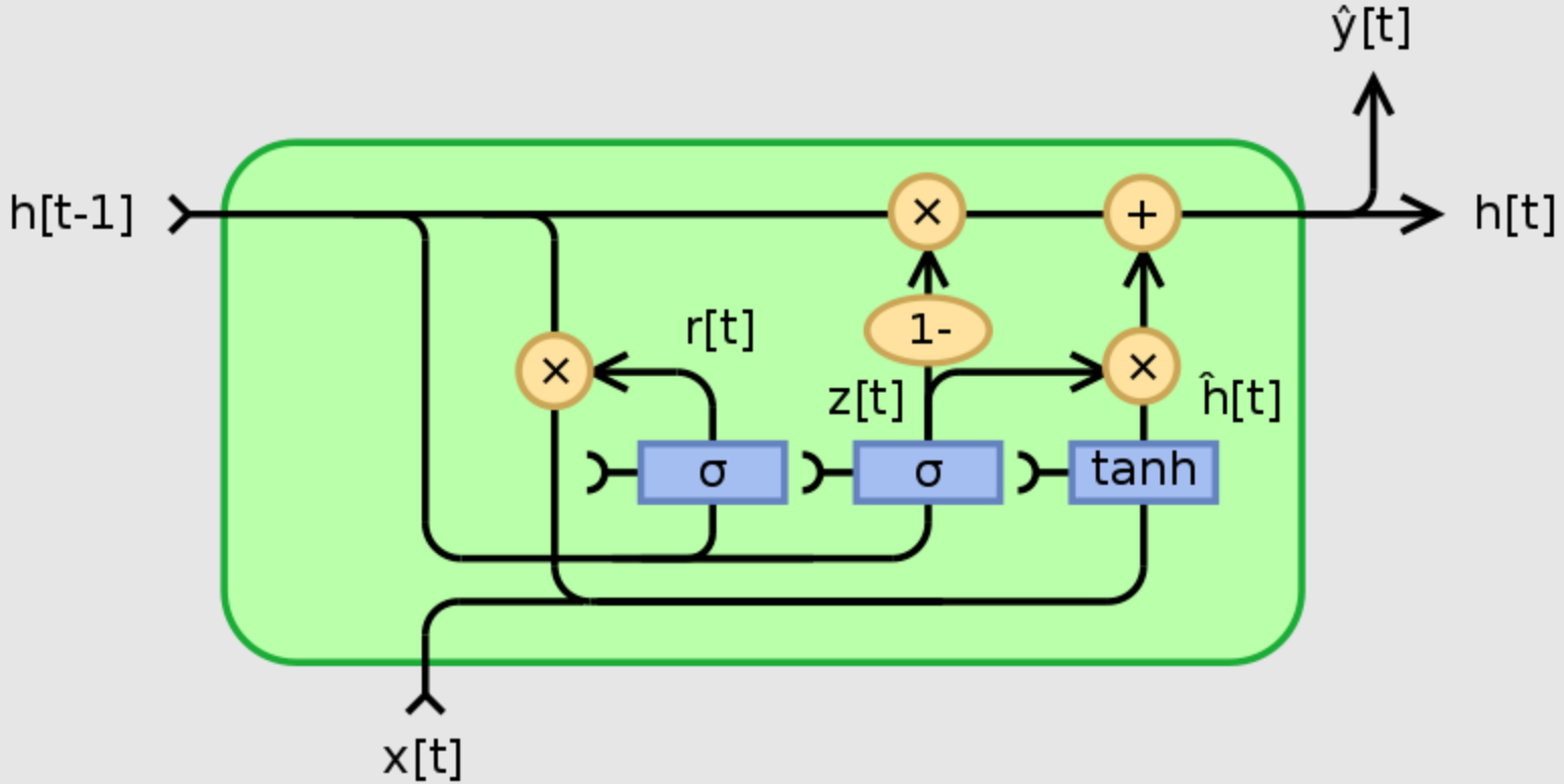
Complexity: LSTMs have a more complex architecture with three gates (forget, input, and output) and a cell state. GRUs have a simpler design with two gates (reset and update) and rely on the hidden state for memory.
Information flow: LSTMs have a clearer separation of controlling information flow. The forget gate decides what to forget from the cell state, the input gate controls new information from the current input, and the output gate determines what the next hidden state will be. GRUs combine these functionalities into their update gate, making them less granular but potentially faster to train.

Strengths and Weaknesses:

LSTMs:
- Strengths: More powerful for capturing long-term dependencies, potentially better performance for complex tasks.
- Weaknesses: More complex and computationally expensive to train, may be prone to overfitting with limited data.
GRUs:
- Strengths: Simpler and faster to train compared to LSTMs, less prone to overfitting.
- Weaknesses: May not be as effective as LSTMs for tasks requiring very long-term dependencies.

Choosing between LSTMs and GRUs:

If your task involves complex sequences and long-term dependencies, LSTMs might be a better choice despite their computational cost.
If your dataset is limited or computational resources are constrained, GRUs can be a good alternative due to their efficiency and ease of training.
In many cases, the best option may not be clear upfront. Experimenting with both LSTMs and GRUs on your specific dataset can help determine which performs better.

Bidirectional RNNs (BRNNs)

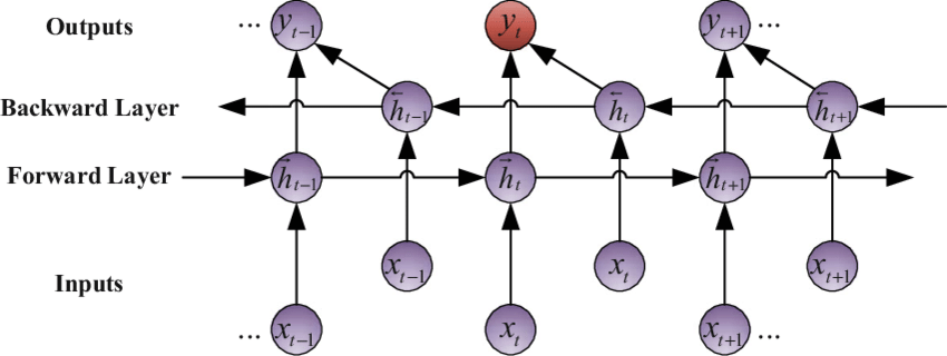
A bidirectional recurrent neural network (BRNN) processes data sequences with forward and backward layers of hidden nodes. The forward layer works similarly to the RNN, which stores the previous input in the hidden state and uses it to predict the subsequent output. Meanwhile, the backward layer works in the opposite direction by taking both the current input and the future hidden state to update the present hidden state. Combining both layers enables the BRNN to improve prediction accuracy by considering past and future contexts. For example, you can use the BRNN to predict the word trees in the sentence Apple trees are tall.

The outputs of the two RNNs are usually concatenated at each time step, though there are other options, e.g. summation. The individual network blocks in a BRNN can either be a traditional RNN, GRU, or LSTM depending upon the use-case.

Strengths and Weaknesses:

Strengths: Captures context from both past and future elements in a sequence, potentially leading to better understanding.
Weaknesses: Can be more complex to train compared to LSTMs due to the double processing, might not always utilize the future context effectively depending on the task.

Choosing between BRNNs and LSTMs:

If the task heavily relies on understanding the full context of a sequence (e.g., sentiment analysis of a sentence, machine translation), BRNNs can be advantageous.
For simpler tasks where only the past or future context matters (e.g., speech recognition, music generation), LSTMs might be sufficient.
BRNNs can also be computationally expensive due to the double processing. If resources are limited, LSTMs might be a better choice.

LLMs Series - Part 3 - RNNs

Overview

Rule-Based Machine Translation (RBMT)

Statistical Machine Translation (SMT)

Neural Machine Translation (NMT)

Recurrent Neural Networks (RNNs)

Long-Short Term Memory (LSTMs)

Step-by-Step LSTM Walkthrough

Gated Recurrent Units (GRUs)

Bidirectional RNNs (BRNNs)

Further Readings

Trending Tags