LLMs Series - Part 2 - Word Embeddings

Overview

In the previous part, we covered how to tokenize the data for training a language model for next word prediction. Tokenization was the first step, now let’s look into word embeddings.

This article aims to answer how the LLM learns word semantics and grammar from the tokenized data fed to it.

Early methods (pre-2010s)

Let’s start with an example, we want to train a LLM that takes a sentence in “English” and translates it to “French”. We will assume we have tons of csv data in the format of (English Sentence, French Sentence) in each line. Now the question is how will you prepare the features from the given data?

Consider a more conventional example where we want to predict the housing price and we have string columns like Area. We typically one-hot encode these features and pass them to the model.

Let’s extend the same logic and try it on the previous example. Say I have a string “How are you?”, I have two options:

• I can encode the whole string using one-hot encoding
  • If I encode the whole sentence, then the number of features is going to explode and the model will see very little data of each feature.
  • So clearly this is not the way to go about this.
• Breakdown the string into words and one-hot encode them
  • This seems like a more plausible option so let’s go ahead and try it

# Simple tokenization example using Python's built-in string functions
text = "How are you?"
tokens = text.split()  # Split the text into tokens based on whitespace
print(tokens)

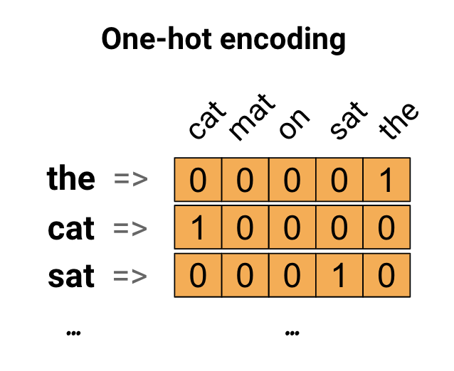
Though the above code is bit of an over simplification, ideally we iterate over all the lines and identify all the unique words. To simplify, let’s say we found about 100 words. Now to represent the word the we define a vector of length 100 where the position corresponding to the is set to 1 and rest are 0.

Now we can extend that logic to a sentence and say, I’ll breakdown the sentence into words and add up the word vectors to represent the sentence. If there is a repetition of words in the sentence, the vector would present the number of occurrences of the same.

But there is still an issue with this method. The sentence How are you will be treated the same as you are how which is a bit absurd. We want the model to learn the grammar and semantic correctly but the feature representing the sentence has no context on the order!

This is another problem that can be quickly addressed by not taking the sum and just stacking the word vectors to form a matrix where the i row represents the i word in the sentence.

Turns out this a pretty good way to prepare text data as features for modelling as was evident in pre-2010s for traditional neural network language models (NNLMs).

But there were a few glaring issues with this technique:

• Struggle to generalize unseen words & contexts
  • The model will be only as good as the data it has seen. If it encounters a new word or a sentence in a different context it’ll be stumped.
  • We say this because the features are the learning tools for the model and if the features don’t capture such info model will not be able to learn.
• Curse of dimensionality
  • Given the high number of words in training data the word vectors are going to be huge, in other words of very high dimensionality
  • This adds its own set of complexities
    • In high-dimensional spaces, data points become increasingly sparse, meaning that the available data becomes more spread out, and the density of data points decreases
    • As the dimensionality of the data increases, the computational complexity of algorithms tends to grow exponentially
    • In high-dimensional spaces, models have a higher tendency to overfit the training data, capturing noise and spurious correlations rather than meaningful patterns
    • Traditional distance metrics such as Euclidean distance become less effective in high-dimensional spaces
    • Storing and processing high-dimensional data can be challenging and resource-intensive

Word Embeddings

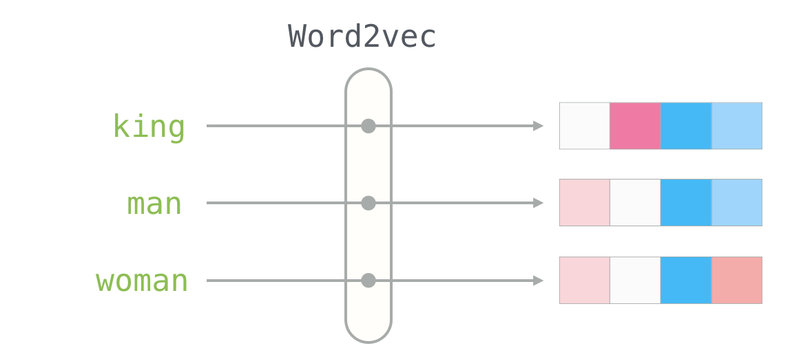
The limitations of previous word tokenization techniques paved the way for one of the most popular technique called Word Embeddings which rose to fame with the word2vec and GloVe. These techniques represented words as dense vectors in a continuous vector space which solved the problem of higher dimensionality prevalent in the one-hot encoding techniques.

This is quite incredible because imagine with word embeddings the machine can do arithmetics on words like king - man + woman = queen !!! Curious to try it out yourself, you can use the snipped below:

from gensim.models import Word2Vec

# Example sentences for training Word2Vec model
sentences = [["king", "man", "woman"], ["queen", "woman", "man"], ["boy", "girl", "man"], ["brother", "sister", "man"]]

# Train Word2Vec model
model = Word2Vec(sentences, vector_size=100, window=5, min_count=1, workers=4)

# Perform word arithmetic: king - man + woman
result = model.wv.most_similar(positive=['king', 'woman'], negative=['man'], topn=1)

# Print the result
print("Result of word arithmetic (king - man + woman):")
print(result)

Word2Vec

Word2Vec is a popular technique used to learn distributed representations of words in a continuous vector space. It is based on the idea that words with similar meanings tend to occur in similar contexts, and these relationships can be captured by the patterns of co-occurrence of words in a large corpus of text.

Here’s an intuitive explanation of how Word2Vec works with an example:

Let’s consider the following two sentences:

1. “The cat sat on the mat.”
2. “The dog slept on the rug.”

Word2Vec learns to represent each word in a fixed-size vector space based on the contexts in which it appears. The key intuition behind Word2Vec is that words appearing in similar contexts should have similar vector representations.

In addition to its utility as a word-embedding method, some of its concepts have been shown to be effective in creating recommendation engines and making sense of sequential data even in commercial, non-language tasks. Companies like Airbnb, Alibaba, Spotify, and Anghami have all benefitted from carving out this brilliant piece of machinery from the world of NLP and using it in production to empower a new breed of recommendation engines.

Vector Representation

Having already looked at one-hot encoding, we know that we can use vectors to represent words for ML models. For one-hot encoding, each column represents a word token and is binary in nature ie, values are 0/1. This leads to a host of disadvantages as mentioned earlier.

What if we reduce the dimensionality and let the ML model figure out what the features should represent and map words to a N-dimensional vector space. For example, let’s say if have model that can convert a word to point in a 2-D space, that will be the vector representation of the word. And this vector can easily be passed to a ML model to represent words. Words that are closer together in the 2-D space would have similar semantic meaning, like king and queen might be mapped close together in the 2-D space by the model because they’re often used in a similar way in sentences.

  1.0 |
      |  (cat)
  0.8 |       (dog)
      |
  0.6 |
      |            (mat)
  0.4 |                (rug)
      |
  0.2 |
      |
  0.0 ---------------------------------
      0.2   0.4   0.6   0.8   1.0

This is exactly what Word2Vec does but with a much larger dimensions (like 50). It maps each word to a dense, low-dimensional vector that captures its semantic meaning. During training, Word2Vec learns the vectors by predicting a word based on its context (surrounding words).

Key Concepts

1. Context Window:
   • Word2Vec considers a fixed-size context window around each word in the corpus. The context window defines the neighbouring words that are considered when learning the representation of a target word.
   • For example, if we choose a context window size of 2, for the word “cat” in the first sentence, the context would be [“the”, “sat”, “on”].
2. Learning Word Representations:
   • Word2Vec uses a neural network architecture, typically a shallow neural network, to learn the word representations.
   • It treats each word in the vocabulary as a target word and tries to predict the surrounding words (context words) within the context window.
   • The network is trained by adjusting the weights such that the predicted context words are close to the actual context words in the vector space.
3. Vector Space Representation:
   • After training, each word in the vocabulary is represented as a dense vector in the learned vector space.
   • Words with similar meanings or usage tend to have vectors that are close together in this space.
   • For example, the vectors for “cat” and “dog” might be close together because they both appear in similar contexts (“the”, “sat/on”, “the”).
4. Semantic Relationships:
   • One of the remarkable properties of Word2Vec embeddings is that they capture semantic relationships between words.
   • For example, in the learned vector space, the vector for “king” might be close to the vector for “queen”, “man” might be close to “woman”, “cat” might be close to “dog”, etc.

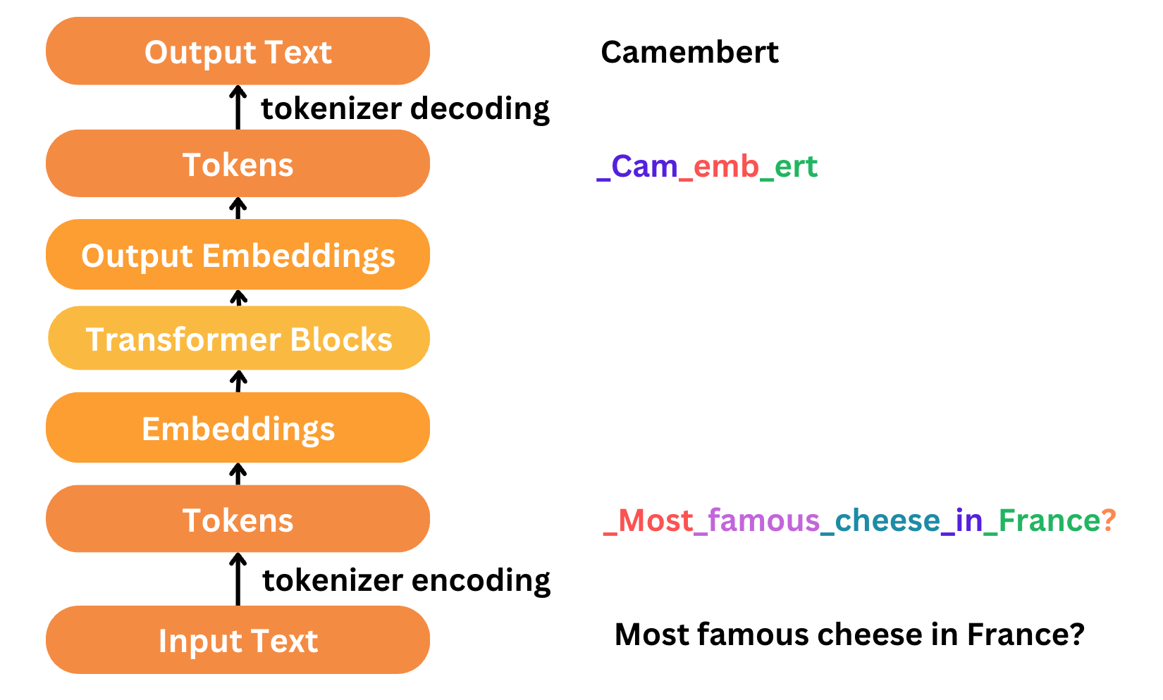
Language Modeling

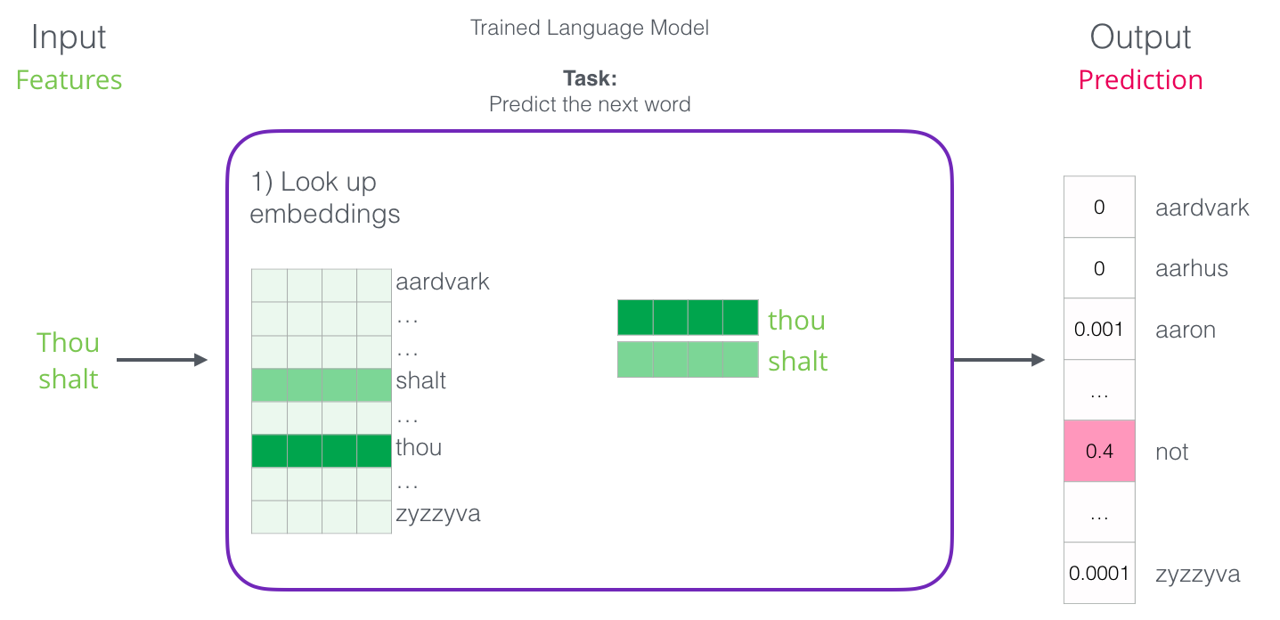
One of the most popular and early applications of NLP was next word prediction. All of us have probably leveraged this capability from our smartphone’s keyboard! Next-word prediction is a task that can be addressed by a language model. A language model can take a list of words (let’s say two words), and attempt to predict the word that follows them.

We can expect a language model to do something as follows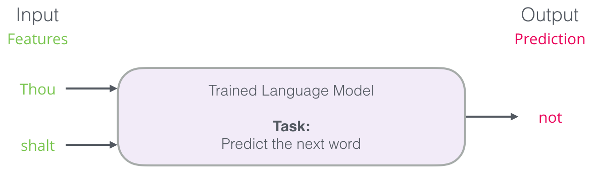

But the machine doesn’t understand words, it outputs probabilities of the possible words. The keyboard application just picks the word with the highest probability and shows it to the user. Combining this information with the vector representation of words, we can say that once we train a language model we can look up embeddings for the input, get a prediction on the output embedding and convert the output embedding to a word!

Language Model Training

Data is the fuel for ML models and is often limited. But in the case of language models, there is plenty of text data to go around.

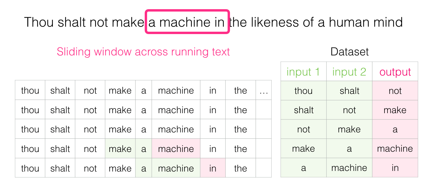
Sliding Window

Words get their embeddings by us looking at which other words they tend to appear next to. The mechanics of that is that

1. We get a lot of text data (say, all Wikipedia articles, for example). then
2. We have a window (say, of three words) that we slide against all of that text.
3. The sliding window generates training samples for our model

As shown in the example below, a simple sentence can give us a lot of training data.

In practice, models tend to be trained while we’re sliding the window. But I find it clearer to logically separate the “dataset generation” phase from the training phase.

Aside from neural-network-based approaches to language modeling, a technique called N-grams was commonly used to train language models. To see how this switch from N-grams to neural models reflects on real-world products, here’s a 2015 blog post from Swiftkey, my favorite Android keyboard, introducing their neural language model and comparing it with their previous N-gram model.

Look both ways

After training, let’s say this line was passed to the model Jay was hit by a ___. The model might look at it and predict bus. But what if the blank I’m trying to fill is as follows Jay was hit by a ___ bus. This completely changes what should go in the blank.

What we learn from this is the words both before and after a specific word carry informational value. It turns out that accounting for both directions (words to the left and to the right of the word we’re guessing) leads to better word embeddings.

Instead of only looking two words before the target word, we can also look at two words after it. This is called a Continuous Bag of Words architecture and is described in one of the word2vec papers [pdf].

input 1	input 2	input 3	input 4	output
by	a	bus	in	red

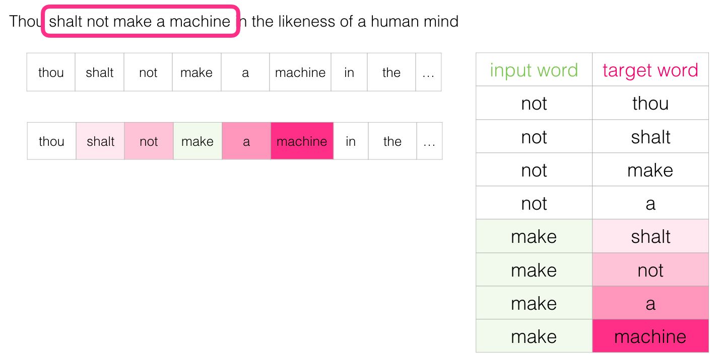
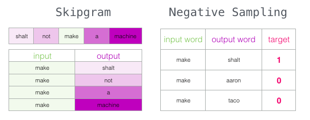
Skip-gram

Instead of guessing a word based on its context (the words before and after it), this other architecture tries to guess neighboring words using the current word. This may sound counter intuitive at first glance but bear with me. Let’s look at how we’ll prepare the data now.

What is the impact of reversing the training pairs?

Consider the sentence “The cat sat on the mat” and the word “sat”:

• With pairs (“sat”, “cat”), (“sat”, “on”), (“sat”, “the”), (“sat”, “mat”):
  • The model learns that “sat” commonly appears with words like “cat”, “on”, “the”, “mat”.
  • If a new sentence uses “sat”, the model can infer that surrounding words may be related to “cat”, “mat”, etc., giving it a strong semantic understanding of “sat”.
• With reversed pairs (“cat”, “sat”), (“on”, “sat”), (“the”, “sat”), (“mat”, “sat”):
  • The model learns to predict “sat” when seeing “cat”, “on”, “the”, “mat”.
  • This teaches the model to expect “sat” in various contexts but doesn’t help it understand what kind of words typically surround “sat”.

Now we have sample data for training, we use a simple neural network with 1 hidden layer for training our language model to predict the next word. We take the input word, generate a one-hot encoded vector and pass it to the model. The model does a forward pass and returns a probability vector. We compute the error against the one-hot encoded vector for the target word and update the gradients.

But this still has it’s challenges!

Breaking it down

Given that we will have massive sizes for the one-hot encoded vectors, computing the error for each and every row in the training set is a huge task computationally and may not be efficient to train a model with such high dimensionality (refer earlier section).

One way around this is to split our target into two steps:

1. Generate high-quality word embeddings (Don’t worry about next-word prediction).
2. Use these high-quality embeddings to train a language model (to do next-word prediction).

We will focus more on #1 since we are interested in word embeddings in the context of this post. So now our goal is to generate word embeddings and to that end our model will look as follows.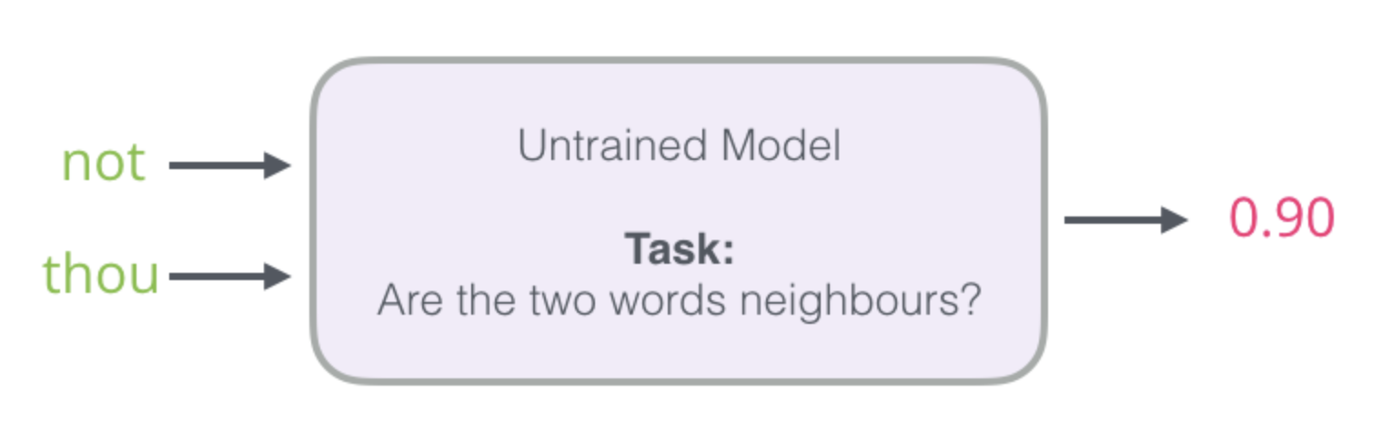

It’ll take a word pair as input and check if the two words are similar. This is also significantly faster since we can now use a simple logistic regression instead of a neural network! But now, how do we prepare the data for such a model then?

Turns out its quite simple and an extension of the previous logic.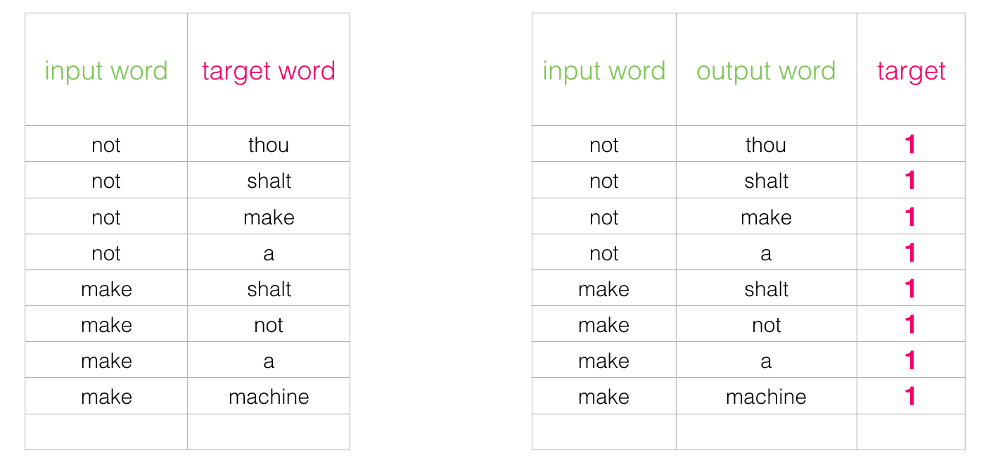

Negative Sampling

Looking at the above diagram we can see a glarring issue with the data we have prepared. All of them have the target as 1 which means that the model can simply predict 1 and forget about the input data to get 100% accuracy!

To address this, we need to introduce negative samples to our dataset – samples of words that are not neighbors. Our model needs to return 0 for those samples. We can generate such samples by randomly picking words from the vocabulary outside the context and mark the target as 0.

This idea is inspired by Noise-contrastive estimation [pdf]. We are contrasting the actual signal (positive examples of neighboring words) with noise (randomly selected words that are not neighbors). This leads to a great tradeoff of computational and statistical efficiency.

word2vec Training Process

Before the training process starts, we pre-process the text we’re training the model against. In this step, we determine the size of our vocabulary (we’ll call this vocab_size, think of it as, say, 10,000) and which words belong to it.

At the start of the training phase, we create two matrices – an Embedding matrix and a Context matrix. These two matrices have an embedding for each word in our vocabulary (So vocab_size is one of their dimensions). The second dimension is how long we want each embedding to be.

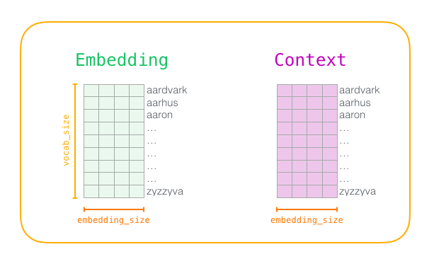
At the start of the training process, we initialize these matrices with random values. Then we start the training process. In each training step, we take one positive example and its associated negative examples.

Once the model is trained, it can be used to generate the word embeddings for an word in the vocabulary it was trained on and it’ll be a vector of size embedding_size

Window Size

The window size in the Skip-gram model refers to the number of context words considered on either side of a target word. It determines how much context around each word is used to train the model.

Small Window Size

• Focused Context: A smaller window size (e.g., 2) means the model only considers words that are very close to the target word. This results in embeddings that capture more syntactic relationships (like “sat” and “on” in “The cat sat on the mat”).
• Less Diverse Information: With a smaller context, the model may miss out on broader, more semantic relationships that might be present further away from the target word.

Large Window Size

• Broader Context: A larger window size (e.g., 10) allows the model to consider words that are further away from the target word. This helps in capturing more semantic relationships and the overall topic of the text.
• More Noisy Context: However, a larger window might include less relevant words, introducing noise into the training data. For example, in a large window size, “cat” might be paired with “rug” in “The cat sat on the mat” and “The dog slept on the rug”, even though they are not directly related.

A typical window size might range from 2 to 10. Smaller windows focus on syntactic relationships, while larger windows capture more semantic meanings.

Number of Negative Samples

Instead of updating the weights for the entire vocabulary, the model only updates for a small subset of “negative” samples (words that do not appear in the context of the target word).

Few Negative Samples

• Less Efficient Learning: Using too few negative samples (e.g., 2-3) might not provide enough contrastive information to the model. The model may not learn effectively to distinguish between relevant and irrelevant words.
• Faster Training: However, fewer negative samples mean faster training because there are fewer updates per iteration.

Many Negative Samples

• Better Discrimination: Using more negative samples (e.g., 15-20) provides more contrastive information, allowing the model to learn better distinctions between relevant and irrelevant context words.
• Slower Training: More negative samples mean slower training due to more updates per iteration. However, the trade-off is often worthwhile as the model learns more robust and meaningful embeddings.

Typically, 5 to 20 negative samples are used. More samples improve learning but increase computational cost.

Further Readings

• https://jalammar.github.io/illustrated-word2vec/
• https://github.com/piskvorky/gensim/blob/develop/gensim/models/word2vec.py
• https://p.migdal.pl/blog/2017/01/king-man-woman-queen-why
• ChatGPT