Deep Learning Basics

Reference

Generative Deep Learning - Chapter 2

Deep Learning

Deep learning is a class of machine learning algorithms that uses multiple stacked layers of processing units to learn high-level representations from unstructured data.

Deep learning differs from the traditional ML models in the sense that the former can learn how to build high-level information by itself from unstructured data. While ML models like Xgboost, logistic regression etc rely on the input features to be informative & not spatially dependent like pixels on a image.

Deep Neural Networks

What is a neural network?

A neural network consists of a series of stacked layers. Each layer contains units that are connected to the previous layer’s units through a set of weights. Neural networks where all adjacent layers are fully connected are called multilayer perceptrons (MLPs).

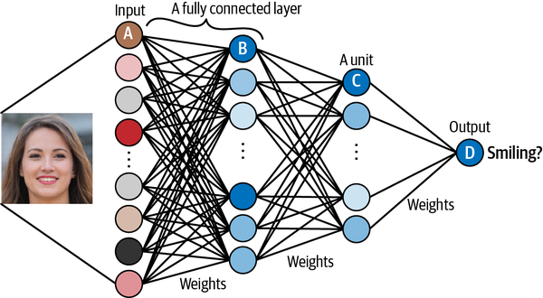
The input (e.g., an image) is transformed by each layer in turn, in what is known as a forward pass through the network, until it reaches the output layer. Specifically, each unit applies a nonlinear transformation to a weighted sum of its inputs and passes the output through to the subsequent layer.

The magic of deep neural networks lies in finding the set of weights for each layer that results in the most accurate predictions.

During the training process, batches of images are passed through the network and the predicted outputs are compared to the ground truth. The error in the prediction is then propagated backward through the network, adjusting each set of weights a small amount in the direction that improves the prediction most significantly. This process is appropriately called backpropagation.

Gradually, each unit becomes skilled at identifying a particular feature that ultimately helps the network to make better predictions.

Learning high-level features

The critical property that makes neural networks so powerful is their ability to learn features from the input data, without human guidance. In other words, we do not need to do any feature engineering, which is why neural networks are so useful! We can let the model decide how it wants to arrange its weights, guided only by its desire to minimize the error in its predictions.

MLP on CIFAR-10 dataset

Multi Layer Perceptron (MLP)

It is a type of feedforward artificial neural network (ANN) composed of multiple layers of nodes (neurons), organized in a sequence of interconnected layers: an input layer, one or more hidden layers, and an output layer.

Here are some key characteristics of MLPs:

1. Feedforward Network: In MLPs, information flows in one direction, from the input layer through the hidden layers (if any) to the output layer. There are no cycles or loops in the connections.

2. Fully Connected Layers: Each node in one layer is connected to every node in the subsequent layer, hence the term “fully connected.” This architecture allows MLPs to capture complex relationships in the data.

3. Non-linear Activation Functions: Typically, each node in the hidden layers and the output layer (except in some cases) applies a non-linear activation function to its input. This introduces non-linearity into the model, enabling it to learn complex patterns in the data.

4. Training with Backpropagation: MLPs are trained using the backpropagation algorithm, which involves calculating gradients of the loss function with respect to the weights of the network and adjusting the weights using gradient descent or its variants.

5. Universal Function Approximators: Theoretically, MLPs with a single hidden layer containing a finite number of neurons can approximate any continuous function to arbitrary accuracy, given a sufficiently large number of neurons.

MLPs have been widely used in various machine learning tasks, including classification, regression, and pattern recognition. However, they may struggle with tasks involving sequential or spatial data, where other architectures like recurrent neural networks (RNNs) or convolutional neural networks (CNNs) might be more suitable.

CIFAR-10 dataset

The CIFAR-10 dataset is a widely used benchmark dataset in the field of computer vision. It stands for Canadian Institute for Advanced Research - 10, indicating that it was collected and labeled by researchers at CIFAR. The dataset consists of 60,000 32x32 color images in 10 classes, with 6,000 images per class. The classes are mutually exclusive and include:

1. Airplane
2. Automobile
3. Bird
4. Cat
5. Deer
6. Dog
7. Frog
8. Horse
9. Ship
10. Truck

CIFAR-10 is often used for image classification tasks, and its relatively small size makes it suitable for testing and prototyping machine learning and deep learning models. It’s also a standard benchmark for evaluating the performance of different algorithms in the computer vision community.

Model Definition

A sample MLP can be defined in pytorch as follows:

class MLP(nn.Module): 
	def __init__(self, input_size, hidden_size, num_classes): 
		super(MLP, self).__init__() 
		self.fc1 = nn.Linear(input_size, hidden_size) 
		self.relu = nn.ReLU() 
		self.fc2 = nn.Linear(hidden_size, num_classes)
		
	def forward(self, x):
		out = self.fc1(x)
		out = self.relu(out)
		out = self.fc2(out)
		return out

This code translates to a neural network as shown in the diagram below: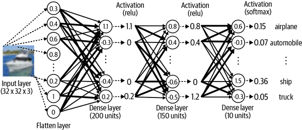

To break down the model further:

• The first layer flattens the 3-D input to a 1-D input
• This is now passed as input to a dense/linear layer with 200 units/neurons. Each arrow has a weight associated with the same and each neuron’s output can be computed as the weighed sum of the input multiplied by the weights.
• The output from the neuron is passed to an activation layer which add non-linearity into the model allowing it to learn complex patterns and relationships in the data
  • If not for non-linear activation layers, the neural network can only model linear relationships but real world problems involve highly non-linear relationships
  • Non-linear activation functions introduce non-linearities at each layer, allowing the network to create hierarchical representations of the input data. This hierarchy enables the network to learn increasingly abstract and complex features as we move deeper into the network.
  • It has been mathematically proven that neural networks with non-linear activation functions are universal function approximators and can approximate any continuous function to a degree of accuracy!
• We are using relu & softmax for activation
  • 
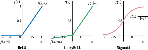
  • The ReLU (rectified linear unit) activation function is defined to be 0 if the input is negative and is otherwise equal to the input.
  • ReLU units can sometimes die if they always output 0, because of a large bias toward negative values pre-activation. In this case, the gradient is 0 and therefore no error is propagated back through this unit. LeakyReLU activations fix this issue by always ensuring the gradient is nonzero.
  • The sigmoid activation is useful if you wish the output from the layer to be scaled between 0 and 1
• Each dense layer is followed by an activation layer for the aforementioned reasons and finally we gather the output via a sigmoid function to model the probability that the img belongs to one of the labels.

Loss Functions

The loss function is used by the neural network to compare its predicted output to the ground truth. It returns a single number for each observation; the greater this number, the worse the network has performed for this observation.

If your neural network is designed to solve a regression problem (i.e., the output is continuous), then you might use the mean squared error loss. This is the mean of the squared difference between the ground truth $y_i$ and predicted value $\hat{y_i}$ of each output unit, where the mean is taken over all $n$ output units: \(\text{MSE} = \frac{1}{n} \sum_{i=1}^{n} (y_i - \hat{y}_i)^2\) If you are working on a classification problem where each observation only belongs to one class, then categorical cross-entropy is the correct loss function. This is defined as follows: \(\text{Categorical Cross Entropy} = -\sum_{i} y_i \log(\hat{y}_i)\) Finally, if you are working on a binary classification problem with one output unit, or a multilabel problem where each observation can belong to multiple classes simultaneously, you should use binary cross-entropy: \(BCE(y, \hat{y}) = -\frac{1}{N} \sum_{i=1}^{N} \left( y_i \cdot \log(\hat{y}_i) + (1 - y_i) \cdot \log(1 - \hat{y}_i) \right)\)

Optimizers

The optimizer is the algorithm that will be used to update the weights in the neural network based on the gradient of the loss function. One of the most commonly used and stable optimizers is Adam (Adaptive Moment Estimation).

In most cases, you shouldn’t need to tweak the default parameters of the Adam optimizer, except the learning rate. The greater the learning rate, the larger the change in weights at each training step. While training is initially faster with a large learning rate, the downside is that it may result in less stable training and may not find the global minimum of the loss function. This is a parameter that you may want to tune or adjust during training.

Another common optimizer that you may come across is RMSProp (Root Mean Squared Propagation).

Code

import torch
import torch.nn as nn
import torchvision
import torchvision.transforms as transforms
from torch.utils.data import DataLoader

## Define the neural network
class MLP(nn.Module):
    def __init__(self, input_size, hidden_size, num_classes):
        super(MLP, self).__init__()
        self.fc1 = nn.Linear(input_size, hidden_size)
        self.relu = nn.ReLU()
        self.fc2 = nn.Linear(hidden_size, num_classes)
    
    def forward(self, x):
        out = self.fc1(x)
        out = self.relu(out)
        out = self.fc2(out)
        return out

## Device configuration
device = torch.device('cuda' if torch.cuda.is_available() else 'cpu')

## Hyperparameters
input_size = 32 * 32 * 3  # CIFAR-10 image size is 32x32x3
hidden_size = 100
num_classes = 10
learning_rate = 0.001
num_epochs = 5
batch_size = 100

## Load CIFAR-10 dataset
transform = transforms.Compose([
    transforms.ToTensor(),
    transforms.Normalize((0.5, 0.5, 0.5), (0.5, 0.5, 0.5))
])

train_dataset = torchvision.datasets.CIFAR10(root='./data', train=True, download=True, transform=transform)
train_loader = DataLoader(dataset=train_dataset, batch_size=batch_size, shuffle=True)

test_dataset = torchvision.datasets.CIFAR10(root='./data', train=False, download=True, transform=transform)
test_loader = DataLoader(dataset=test_dataset, batch_size=batch_size, shuffle=False)

## Initialize the model
model = MLP(input_size, hidden_size, num_classes).to(device)

## Loss and optimizer
criterion = nn.CrossEntropyLoss()
optimizer = torch.optim.Adam(model.parameters(), lr=learning_rate)

## Training the model
total_step = len(train_loader)
for epoch in range(num_epochs):
    correct = 0
    total = 0
    for i, (images, labels) in enumerate(train_loader):
        # Move tensors to the configured device
        images = images.reshape(-1, input_size).to(device)
        labels = labels.to(device)
        
        # Forward pass
        outputs = model(images)
        loss = criterion(outputs, labels)
        
        # Backward pass and optimize
        optimizer.zero_grad()
        loss.backward()
        optimizer.step()
        
        # Track the accuracy
        _, predicted = torch.max(outputs.data, 1)
        total += labels.size(0)
        correct += (predicted == labels).sum().item()
        
        if (i+1) % 100 == 0:
            print ('Epoch [{}/{}], Step [{}/{}], Loss: {:.4f}, Accuracy: {:.2f} %' 
                   .format(epoch+1, num_epochs, i+1, total_step, loss.item(), (correct/total)*100))

## Test the model
model.eval()  
with torch.no_grad():
    correct = 0
    total = 0
    for images, labels in test_loader:
        images = images.reshape(-1, input_size).to(device)
        labels = labels.to(device)
        outputs = model(images)
        _, predicted = torch.max(outputs.data, 1)
        total += labels.size(0)
        correct += (predicted == labels).sum().item()

    print('Accuracy of the network on the 10000 test images: {} %'.format(100 * correct / total))

Most of the code is self-explanatory so we’ll go into the details for just a few lines.

• optimizer.zero_grad()
  • This function clears (zeroes) the gradients of all optimized parameters.
  • In PyTorch, gradients are accumulated by default whenever .backward() is called on a tensor.
  • Before computing gradients for the next minibatch of training data, it’s essential to zero out the gradients from the previous minibatch.
  • Otherwise, gradients would accumulate, leading to incorrect results.
• loss.backward()
  • This function computes gradients of the loss with respect to all parameters that have requires_grad=True.
  • It effectively calculates the gradients of the loss function with respect to each parameter of the model.
  • These gradients are then used to update the parameters during optimization.
• optimizer.step()
  • This function updates the parameters of the model based on the gradients computed in the backward() pass.
  • It applies the optimization algorithm (e.g., SGD, Adam) to adjust the parameters in the direction that minimizes the loss.
  • Essentially, it takes a step in the opposite direction of the gradient to minimize the loss function.
• model.eval
  • This method sets the model to evaluation mode. During evaluation, we don’t want certain layers (like dropout or batch normalization) to behave differently than during training.
  • For example, dropout layers are typically used during training to prevent overfitting by randomly dropping some activations, but during evaluation, we want the full strength of the model. model.eval() ensures that the model is set up correctly for evaluation by disabling such layers or operations that behave differently during training.
• torch.no_grad()
  • This context manager is used to temporarily set all requires_grad flags to False. When performing inference or evaluation, we don’t need to compute gradients because we’re not updating the model’s parameters.
  • Disabling gradient tracking using torch.no_grad() reduces memory consumption and speeds up computations by avoiding the computation of unnecessary gradients during inference.
  • It ensures that operations inside the context manager do not build the computational graph required for gradient computation.

Evaluation

Final evaluation of the trained model on the test dataset, show that accuracy of the network on the test dataset is 49.96 %

Let’s see if we can do better.

CNN on CIFAR-10 dataset

One of the reasons our network isn’t yet performing as well as it might is because there isn’t anything in the network that takes into account the spatial structure of the input images. In fact, our first step is to flatten the image into a single vector, so that we can pass it to the first Dense layer!

Convolutional Layers

The figure below shows two different 3 × 3 × 1 portions of a grayscale image being convoluted with a 3 × 3 × 1 filter (or kernel). The convolution is performed by multiplying the filter pixelwise with the portion of the image, and summing the results. The output is more positive when the portion of the image closely matches the filter and more negative when the portion of the image is the inverse of the filter. The top example resonates strongly with the filter, so it produces a large positive value. The bottom example does not resonate much with the filter, so it produces a value near zero.

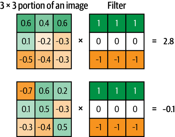
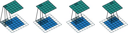
If we move the filter across the entire image from left to right and top to bottom, recording the convolutional output as we go, we obtain a new array that picks out a particular feature of the input, depending on the values in the filter.

A convolutional layer is simply a collection of filters, where the values stored in the filters are the weights that are learned by the neural network through training. Initially these are random, but gradually the filters adapt their weights to start picking out interesting features such as edges or particular color combinations.

Sample convolution layer in pytorch:

nn.Conv2d(in_channels=3, out_channels=32, kernel_size=3, stride=1, padding=1)

In Channels

• This specifies the number of input channels, which corresponds to the number of color channels in the input image (3 for RGB).

Out Channels

• This specifies the number of output channels, which corresponds to the number of filters (or kernels) applied in this layer.

Kernel Size

• The kernel_size parameter determines the size of the convolutional filter or kernel. It’s usually specified as a single integer or a tuple (height, width).
• For example, kernel_size=3 means a 3x3 convolutional filter will be used.

Stride

• Stride refers to the number of pixels the filter moves across the input image.
• A stride of 1 (default) means the filter moves one pixel at a time.
• Increasing the stride reduces the spatial dimensions of the output feature map.

Padding

• Padding refers to the number of pixels added to an input image when it is being processed by the convolutional layer.
• It helps to preserve the spatial dimensions of the input volume.
• Padding is usually specified as either ‘valid’ or ‘same’.
  • ‘valid’: No padding (default behavior).
  • ‘same’: Add padding so that the output feature map has the same spatial dimensions as the input.
• Additionally, you can specify the amount of padding explicitly using the padding parameter.

Stacking Convolution Layers

The output of a Conv2D layer is another four-dimensional tensor, now of shape (batch_size, height, width, filters), so we can stack Conv2D layers on top of each other to grow the depth of our neural network and make it more powerful.

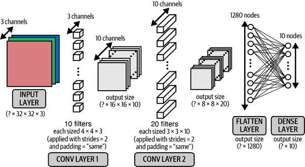
Note that now that we are working with color images, each filter in the first convolutional layer has a depth of 3 rather than 1 (i.e., each filter has shape 4 × 4 × 3, rather than 4 × 4 × 1). This is to match the three channels (red, green, blue) of the input image. The same idea applies to the filters in the second convolutional layer that have a depth of 10, to match the 10 channels output by the first convolutional layer.

Batch Normalization

One common problem when training a deep neural network is ensuring that the weights of the network remain within a reasonable range of values—if they start to become too large, this is a sign that your network is suffering from what is known as the exploding gradient problem. As errors are propagated backward through the network, the calculation of the gradient in the earlier layers can sometimes grow exponentially large, causing wild fluctuations in the weight values.

This doesn’t necessarily happen immediately as you start training the network. Sometimes it can be happily training for hours when suddenly the loss function returns NaN and your network has exploded. This can be incredibly annoying. To prevent it from happening, you need to understand the root cause of the exploding gradient problem.

Covariate Shift

One of the reasons for scaling input data to a neural network is to ensure a stable start to training over the first few iterations. Since the weights of the network are initially randomized, unscaled input could potentially create huge activation values that immediately lead to exploding gradients. For example, instead of passing pixel values from 0–255 into the input layer, we usually scale these values to between –1 and 1.

Because the input is scaled, it’s natural to expect the activations from all future layers to be relatively well scaled as well. Initially this may be true, but as the network trains and the weights move further away from their random initial values, this assumption can start to break down. This phenomenon is known as covariate shift.

Training using batch normalization

During training, a batch normalization layer calculates the mean and standard deviation of each of its input channels across the batch and normalizes by subtracting the mean and dividing by the standard deviation.

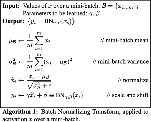
There are then two learned parameters for each channel, the scale (gamma) and shift (beta). The output is simply the normalized input, scaled by gamma and shifted by beta. We can place batch normalization layers after dense or convolutional layers to normalize the output.

Prediction using Batch Normalization

When it comes to prediction, we may only want to predict a single observation, so there is no batch over which to calculate the mean and standard deviation. To get around this problem, during training a batch normalization layer also calculates the moving average of the mean and standard deviation of each channel and stores this value as part of the layer to use at test time.

m = nn.BatchNorm2d(100, momentum=0.9)

The momentum parameter is the weight given to the previous value when calculating the moving average and moving standard deviation.

Dropout

Any successful machine learning algorithm must ensure that it generalizes to unseen data, rather than simply remembering the training dataset. If an algorithm performs well on the training dataset, but not the test dataset, we say that it is suffering from overfitting. To counteract this problem, we use regularization techniques, which ensure that the model is penalized if it starts to overfit.

Dropout layers are a very common technique used for regularization in deep learning. Dropout layers are very simple. During training, each dropout layer chooses a random set of units from the preceding layer and sets their output to 0.

Dropout layers are used most commonly after dense layers since these are the most prone to overfitting due to the higher number of weights, though you can also use them after convolutional layers.

Model Definition

Now let’s look at how a basic CNN would look like.

import torch
import torch.nn as nn

class CNN(nn.Module):
    def __init__(self, num_classes):
        super(CNN, self).__init__()
        self.conv1 = nn.Conv2d(3, 32, kernel_size=3, stride=1, padding=1)
        self.bn1 = nn.BatchNorm2d(32)
        self.relu1 = nn.LeakyReLU()

        self.conv2 = nn.Conv2d(32, 32, kernel_size=3, stride=2, padding=1)
        self.bn2 = nn.BatchNorm2d(32)
        self.relu2 = nn.LeakyReLU()

        self.conv3 = nn.Conv2d(32, 64, kernel_size=3, stride=1, padding=1)
        self.bn3 = nn.BatchNorm2d(64)
        self.relu3 = nn.LeakyReLU()

        self.conv4 = nn.Conv2d(64, 64, kernel_size=3, stride=2, padding=1)
        self.bn4 = nn.BatchNorm2d(64)
        self.relu4 = nn.LeakyReLU()

        self.flatten = nn.Flatten()
        
        self.fc1 = nn.Linear(64 * 8 * 8, 128)
        self.bn5 = nn.BatchNorm1d(128)
        self.relu5 = nn.LeakyReLU()
        self.dropout = nn.Dropout(0.5)
        
        self.fc2 = nn.Linear(128, num_classes)

    def forward(self, x):
        x = self.relu1(self.bn1(self.conv1(x)))
        x = self.relu2(self.bn2(self.conv2(x)))
        x = self.relu3(self.bn3(self.conv3(x)))
        x = self.relu4(self.bn4(self.conv4(x)))
        x = self.flatten(x)
        x = self.relu5(self.bn5(self.fc1(x)))
        x = self.dropout(x)
        x = self.fc2(x)
        return x

## Create the model
model = CNN(num_classes=10)

Evaluation

Final evaluation of the trained model on the test dataset, show that accuracy of the network on the test dataset is 75.52 %

This improvement has been achieved simply by changing the architecture of the model to include convolutional, batch normalization, and dropout layers. Notice that the number of parameters is actually fewer in our new model than the previous model, even though the number of layers is far greater.

This demonstrates the importance of being experimental with your model design and being comfortable with how the different layer types can be used to your advantage. When building generative models, it becomes even more important to understand the inner workings of your model since it is the middle layers of your network that capture the high-level features that you are most interested in.